Workflows
lambda implements different methods to detect seismic or infrasound phases interactively by an operator. As a result slowness, backazimuth and arrival time of the detected phase or time and location of an origin are determined. If possible phase hints are added. The set of configuration parameters is available in the lambda description. Read the section Setup and customization for more details.
Hint
Multiple processing and parameter widgets are available in lambda. Read the section on Widget arrangement for learning how to select and arrange these widgets interactively.
Usual array analysis in lambda consists of
Selection of
data and event if available,
Data pre-processing including filtering as described in section Interactive data processing.
Application of array methods for signal detection to one or more arrays or 3C stations as described in the following sections:
Joint analysis of the detections in the cart of lambda: phase selection and relocation,
Selection and committing the solutions in the cart.
Single time-window detection
The data can be processed in s single time window which is to be selected specifically. Within the time window one of the methods described below can be applied typically results in a single detection which can be selected, analysed and provided to further processing. Besides classical beam methods, lambda also provides conventional phase picking similar to scolv but also 3-component (3C) polarization analysis.
Note
The methods for single time-window analysis are started by pressing buttons in the upper trace window of the Waveform widget.
Phase picking
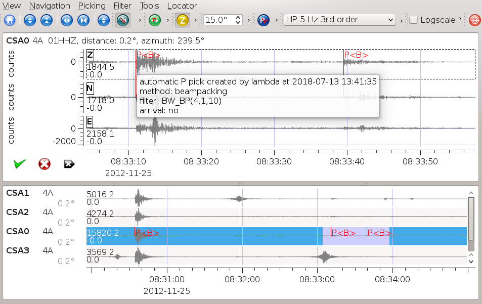
You may interactively pick phase arrival times on single 1C or 3C stations. The arrival times may be added to the cart together with previously determined backazimuth and slowness.
Empty current beam parameters unless you wish to apply them to the new pick. Backazimuth and slowness values may be measured for a specific time window by any of the described workflows: Interactive beamforming, 3C-polarization analysis, 3C-polarization analysis. FK/BP, or PMCC.
Select the traces of a single station or toggle to the beam trace to set the arrival time on the beam trace.
Select a phase type.
Make a pick: double-click with mouse on trace.
Optionally: Set uncertainty by dragging the triangles.
Add pick to Cart for using it or remove the pick.
Continue in Cart to commit the pick to the SeisComP messaging or consider the pick for locating.
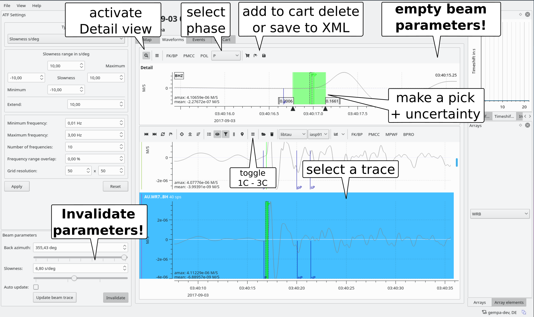
Add phase picks with time, backazimuth, slowness
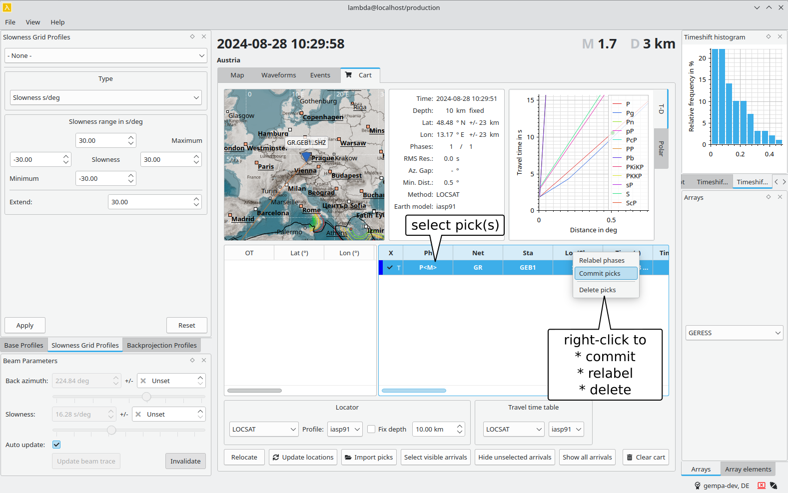
Commit to messaging, delete or relabel picks in cart
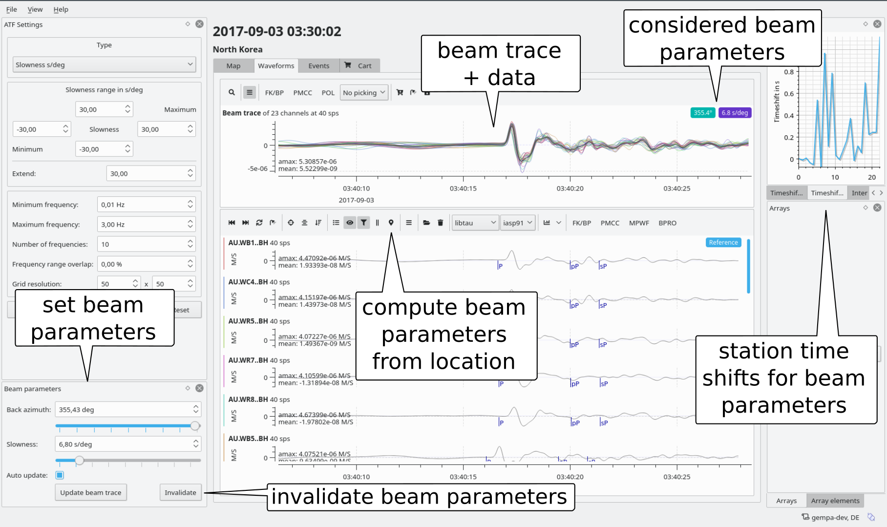
Interactive beamforming
Values for slowness and backazimuth can be provided manually. Then the beam is be formed from the loaded waveforms. The beam is shown in the upper zoom trace widget along with the traces of the stations.
Open Beam parameters window and Timeshift plot: View -> Windows.
Select frequency range in ATF Settings window, press Apply.
Toggle data filtering: press Filter button.
Adjust backazimuth and slowness in Beam parameters window. The corresponding time shifts can be viewed in the window named Timeshift plot.
Make a new pick on a single station or the beam trace (assigned to the reference station). The new pick will receive the measured backazimuth and slowness.
Selection of analysis methods and parameters.
3C-polarization analysis
Instead of using multi-station arrays, the arrival time, backazimuth and incidence
angle can be measured on 3-component (3C) station. Given an effective velocity  of
the uppermost Earth layer, the horizontal slowness
of
the uppermost Earth layer, the horizontal slowness  is derived
from the incidence angle
is derived
from the incidence angle  :
:
(1)
Select a 3C station - may be the same as for picking,
Activate Detail view,
Adjust the time window,
Click on POL,
Adjust values,
Optional: Export ascii file for custom processing,
Press Apply,
Make a new pick on a single station or the beam trace (assigned to the reference station). The new pick will receive the measured backazimuth and slowness.
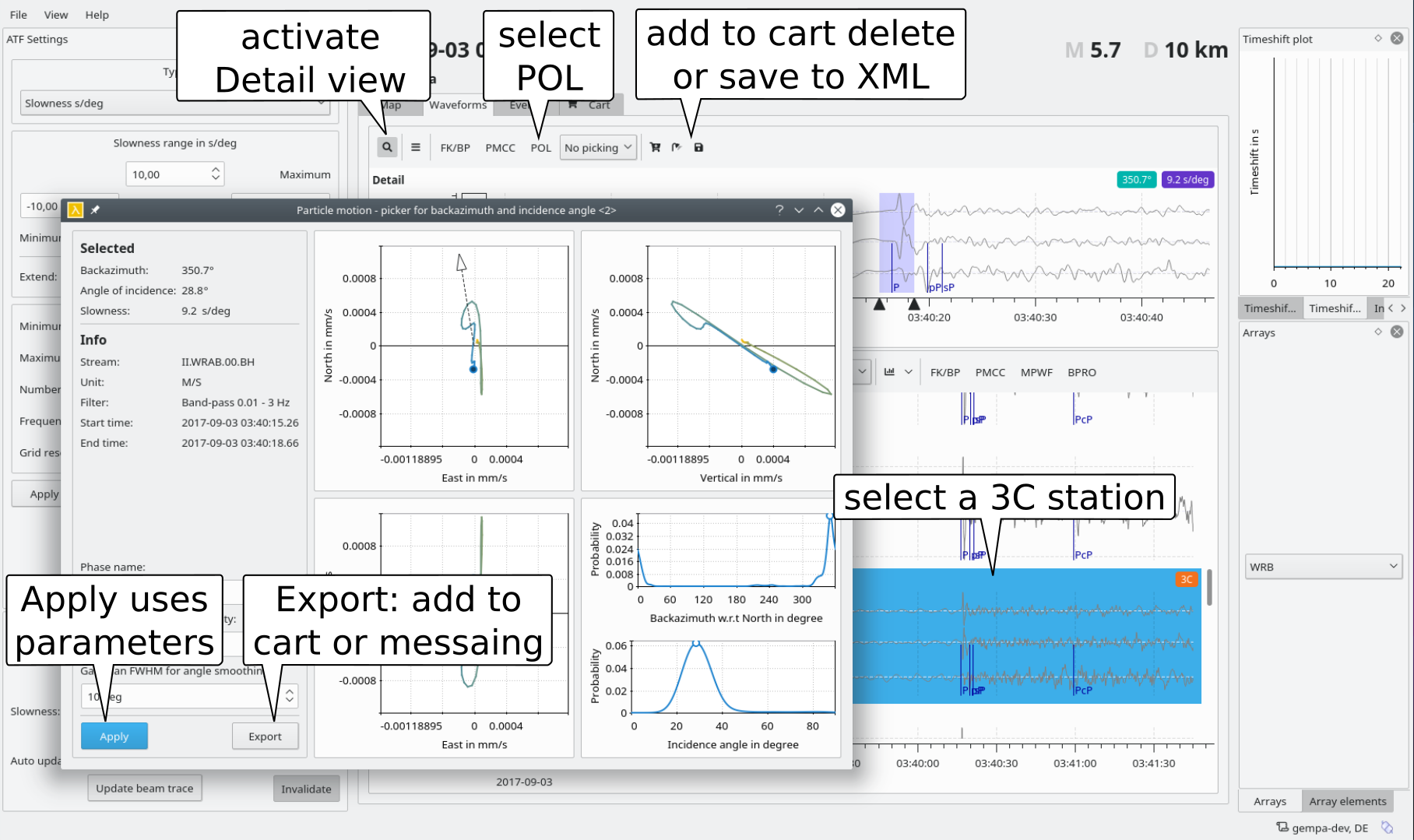
3C polarization analysis.
FK/BP
FK/BP for single time-window analysis to determine slowness and backazimuth by FK or beampacking (BP). The methods are described in the sections F-K analysis and Beampacking.
Select many or all traces: Press A.
Upper trace window: Set the time window large enough. Alternatively, set the slowness range small enough in the window for slowness-grid profiles.
Press ‘FK/BP’ to compute backazimuth and slowness.
optionally review and modify the method and/or sample rate and press Start to repeat the computation.
Press ‘Apply’ to apply backazimuth and slowness to form a new beam.
Make a new pick on a single station or the beam trace (assigned to the reference station). The new pick will receive the measured backazimuth and slowness.
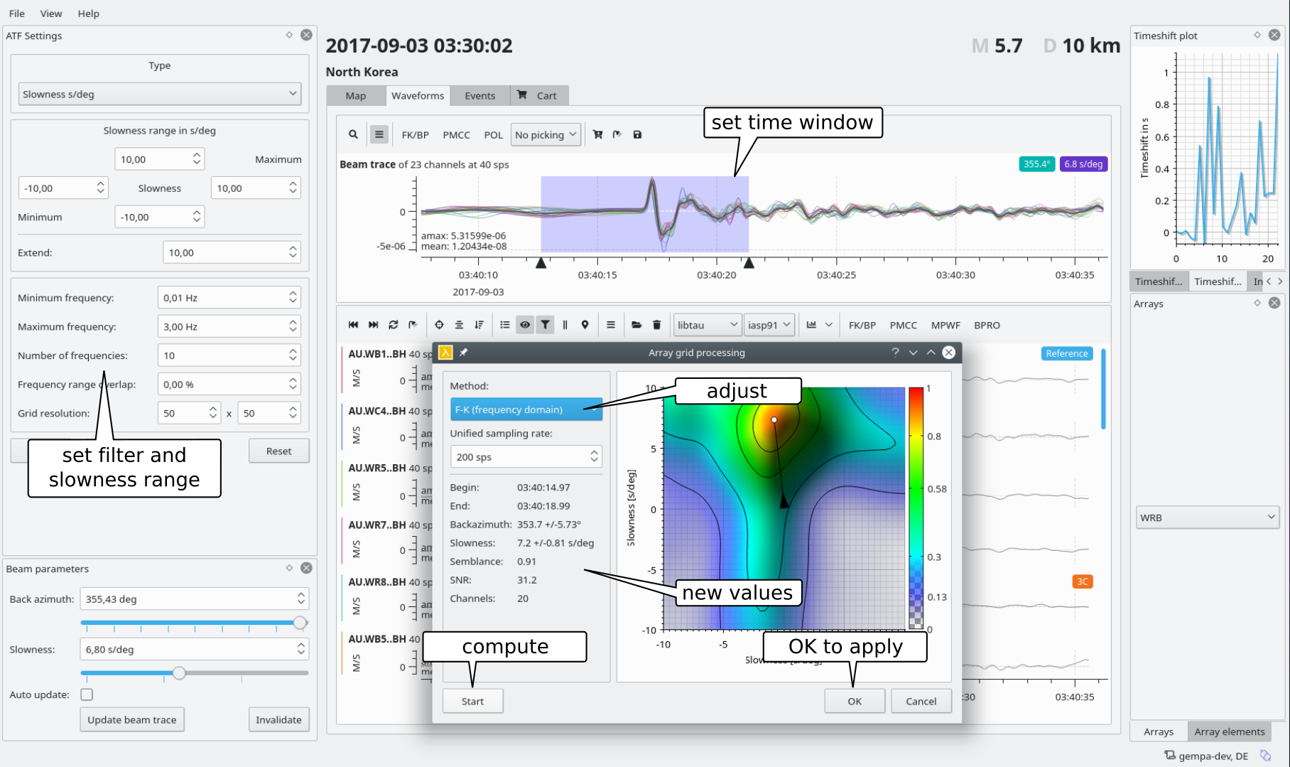
Slowness - backazimuth analysis in single time window.
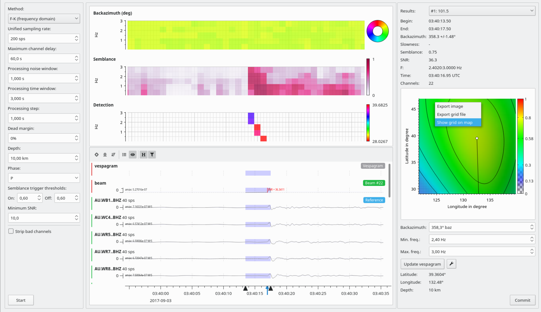
PMCC
Select PMCC for single time-window analysis to determine slowness and backazimuth. The PMCC method is described in section PMCC.
Select many or all traces: Press A.
Upper trace window: Set the time window large enough. Alternatively, set the slowness range small enough in the window for slowness-grid profiles.
Press ‘PMCC’ to compute backazimuth and slowness by PMCC.
optionally review and modify the sample rate and press Start to repeat the computation.
Press ‘Apply’ to apply backazimuth and slowness to form a new beam.
Make a new pick on a single station or the beam trace (assigned to the reference station). The new pick will receive the measured backazimuth and slowness.
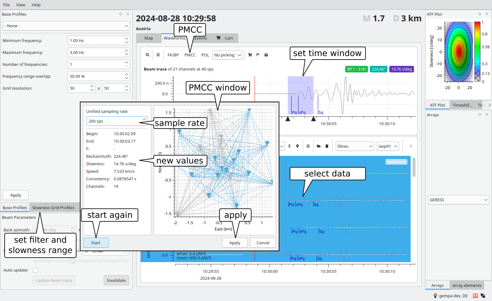
PMCC analysis in single time window.
Sliding time-window detection
The data can be processed continuously by shifting time windows over a longer time series. Within a time window one of the methods described below can be applied. Sliding-time window processing typically results in multiple detections which can be individually selected, analysed and provided to further processing.
Select the data,
Adjust and apply the processing parameters,
Select travel time parameters, e.g. for backprojection or phase hints,
Start a method. The methods for sliding time-window analysis are started with buttons in the lower trace window of the Waveform widget.
Prepare data and select a method.
Inversion of manual picks
The arrival times of manually picked phases can be inverted for slowness, backazimuth and arrival time at the reference station. The plane-wave fitting method is applied.
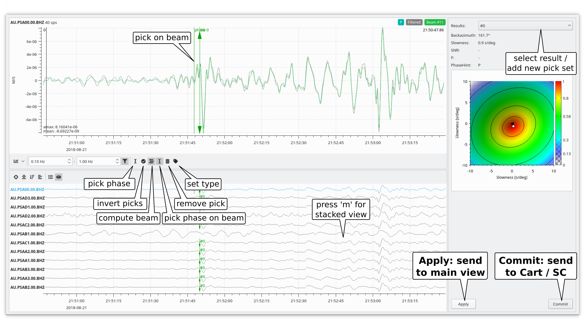
Phase picking and inversion in plane-wave fitting window. Derived values are shown in the upper right. For comparison the contour plot indicates the semblance prediction based on the derived parameters. The maximum should be close the derived value.
Start the manual data processing by clicking on the MPWF button for manual plane-wave fitting in the Waveform widget,
Prepare the data:
Zoom in to the desired time window. The upper pick window can be controlled separately from the lower overview window,
Apply filtering by clicking on the filter button,
Press m to toggle the stacked view,
View spectrograms for enhancing visibility,
Start picking by pressing 1 or by clicking on the pick icon:
Minima or maxima can be picked automatically based on the amplitude extrema. For picking the extrema, drag the time window on the upper pick trace with the mouse. This generally results in very accurate phase picks but the absolute arrival time is delayed. Therefore, later picking on the beam trace is available.
To set picks manually at the arrival time click on the upper trace in the pick window.
Pick multiple traces: Scroll though the traces using the mouse wheel or the arrow up and arrow down keys,
Invert the picks for beam parameters,
Set pick on the beam trace if required,
Optionally: Select New set in the pull down Result selection menu to start another pick set and repeat picking and inversion,
After inversion chose and review a pick set can be chosen in the pull down selection menu,
Integrate the solutions in any of the possible ways:
Press the Apply button to apply the solution in the main lambda window,
Press Commit and Add to cart to provide the solution to the cart,
Press Commit and Send to send picks to the SeisComP system,
Press Commit and check the box Send as artifical origin to send picks with an artificial origin to the SeisComP system. Open the new origin, e.g. in scolv for further process the solution.
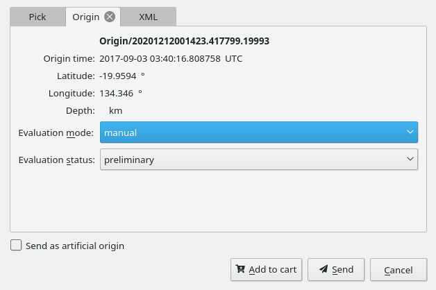
Add picks to cart or send an artificial origin.
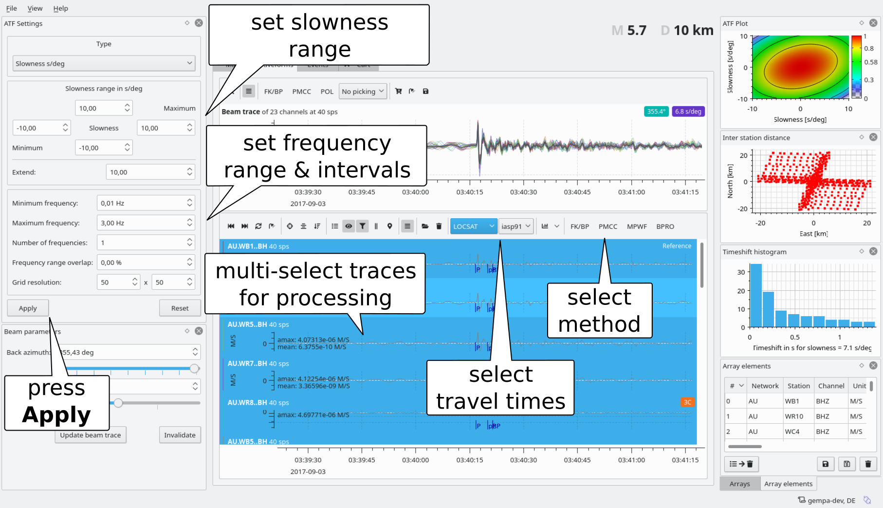
Slowness - wavenumber analysis
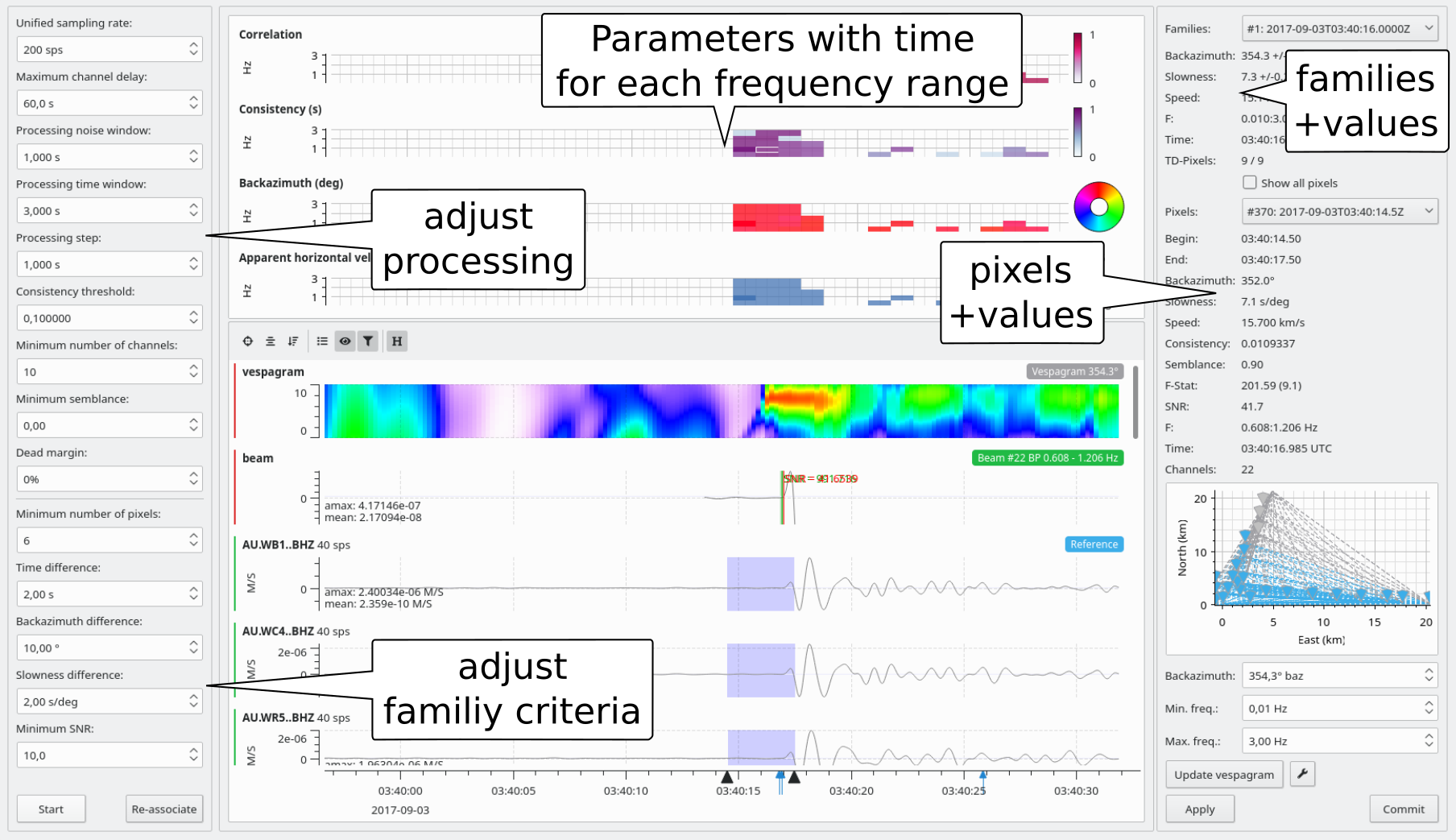
Once the data are loaded and pre-processed the phases can be detected based on slowness / wavenumber analysis. The methods F-K analysis and Beampacking are available.
In the Waveforms window select the type in the Type window along with the slowness / wavenumber ranges. Click on Apply finalize the selection.
For choosing the slowness / wavenumber analysis, double-click on the button for phase detection in the Waveforms window. An new window will open which can be use simultaneously.
For detection set the following parameters in the new window:
Method: Choose F-K analysis or beampbacking for detection.
Unified sampling rate: The sampling interval of the data should not be larger than the differential time shifts between pairs of stations. Therefore the data can be resampled to to a unified sampling rate. Upsampling and downsampling may be useful for small-aperture arrays ad large-aperture arrays, respectively. The sampling rate depends on the array geometry as well as on the slowness and the frequency of the expected signals. Upsampling increases the accuracy of beam packing but slows down the analysis.
Maximum channel delay: Time delay allowing to wait for complete data.
Noise window: Length of noise window used before detection to calculate the SNR
Processing time window: Length of data processing window used for stacking.
Processing step: Time increment between 2 subsequent processing time windows.
Semblance trigger thresholds: Threshold of semblance to declare a detection.
Minium SNR: Minimum SNR which must be reached at the position of the AIC detection for declaring a pick.
To start the analysis, click the start button. When the compuation is finished, the semblance and the beam traces will be shown along with the beam detections. Beam detections are plotted on top of semblance, slowness, backazimuth representing maximum values for each time step.
Select the detection result for reviewing. The selected detection is highlighted in the slowness plot by changing the color. The corresponding beam parameters are shown to the right. The pick and waveform parameters update automatically when selecting another detection. The beam waveform is computed based on the beam parameters. The phase pick is found on the beam trace using the AIC method. It is associated to the reference station of the array.
Compare the detection diagram with the array response function (ATF) for identifying the minor maxima which may be caused by the ATF. For showing the ATF on top of the detection diagram, right click on the diagram and choose “Show ATF contours”. The color of the circles on the contour indicate the semblance level of the contour. Right-click on the detection diagram for saving it to a file.
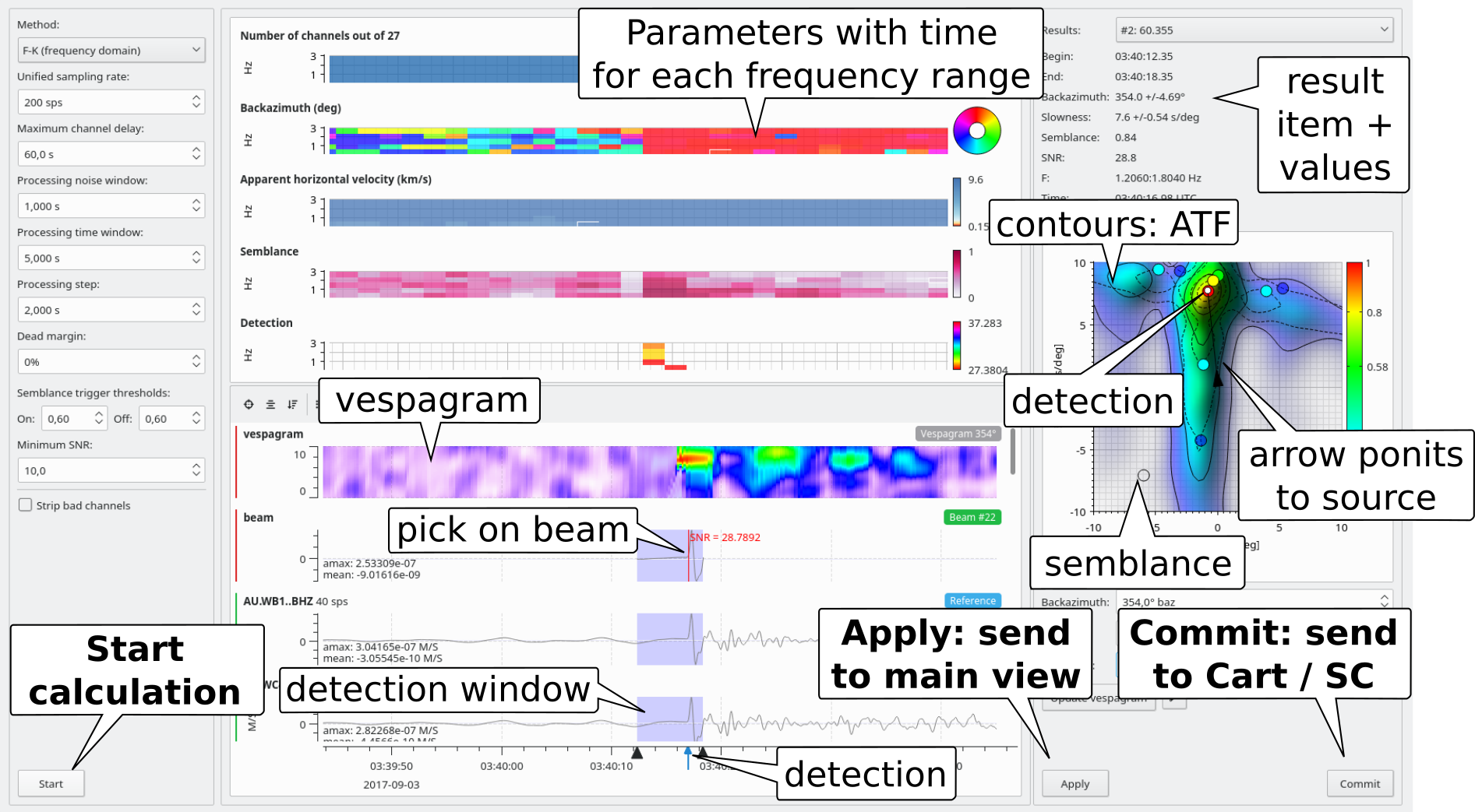
Interactive beam packing window.
To send the pick to the cart or to the SeisComP messaging click on “Commit”. This will open the inspector window in which the pick parameters and the pick XML code can be inspected. After inspection click on the “Send” button to eventually send the parameters or cancel the operation.
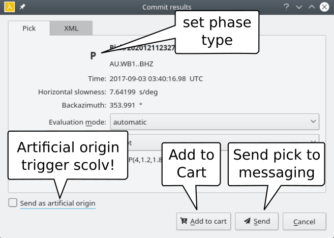
Inspector window showing some details of the solution to be committed.
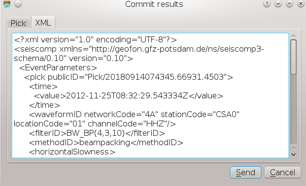
Inspector window showing the full list of objects to be committed in scml.
After sending the pick is available in the SeisComP system and can be used for further analysis. E.g. it can be used for relocating events in scolv. As the beam pick is associated to the reference station of the array it can also be viewed there. The beam pick can be identified by the method B.
Beam pick in the scolv picker window.
PMCC
PMCC is available for sliding time-window analysis. The PMCC method is applied.
Select PMCC in the lower trace window of the Waveform widget for sliding time-window analysis.
Adjust the processing parameters as for Slowness - wavenumber analysis.
Adjust the family criteria as well to join solutions belonging to the same phase.
Press Start to calculate the parameters.
Select a family.
Apply or commit the solution of the selected family and send to cart or to the SeisComP messaging.
PMCC: Sliding time-window analysis.
Backprojection
lambda can also be used to detect and to locate an earthquake at the same time. The back projection method is applied based on waveform stacking along pre-defined traveltime curves for given source points.
Array widget or Map window: Select the array.
Location grid or map widget: Select the range of the location grid by manually entering the values or by selection on the map on the map. The grid resolution is adapted from the ATF settings widget.
Finally, press Apply.

Map window and Location grid widget: Define the location grid.
Waveform window:
Choose the array and the waveform data
Select the traveltime interface and the traveltime table for calculating the traveltime from each grid point to each array element.
For starting the backprojection analysis, double-click on the BPRO button for backprojection. An new window Backprojection widget will open which can be use simultaneously.
Backprojection widget:
For detection and location set the following parameters:
Method: Choose F-K analysis or beampbacking
Unified sampling rate: The sampling interval of the data should not be larger than the differential time shifts between pairs of stations. Therefore the data can be resampled to to a unified sampling rate. Upsampling and downsampling may be useful for small-aperture arrays ad large-aperture arrays, respectively. The sampling rate depends on the array geometry as well as on the slowness and the frequency of the expected signals. Upsampling increases the accuracy of beam packing but slows down the analysis.
Maximum channel delay: Time delay allowing to wait for complete data.
Noise window: Length of noise window used before detection to calculate the SNR
Processing time window: Length of data processing window used for stacking.
Processing step: Time increment between 2 subsequent processing time windows.
Depth: Depth in kilometer at which the event is search for within the location grid.
Semblance trigger thresholds: Threshold of semblance to declare a detection.
Minium SNR: Minimum SNR which must be reached at the position of the AIC detection for declaring a pick.
To start the analysis, click the Start button. When the computation is finished, the semblance and the beam traces will be shown along with the beam detections. Beam detections are plotted on top of semblance, slowness, backazimuth representing maximum values for each time step.
Select the detection result for reviewing. The selected detection is highlighted in the slowness plot by changing the color. The corresponding origin and beam parameters are shown to the right. The parameters and waveforms update automatically when selecting another result. The beam waveform is computed based on the computed beam parameters for the reference station. The phase pick is found on the beam trace using the AIC method. It is associated to the reference station of the array.
Processing window for beampacking with results.
To send the origin with the pick to the cart or the SeisComP messaging system click on “Commit”. Committing opens the inspector window in which the origin parameters and the pick XML code can be inspected. After inspection click on the “Send” button to eventually send the parameters or cancel the operation.
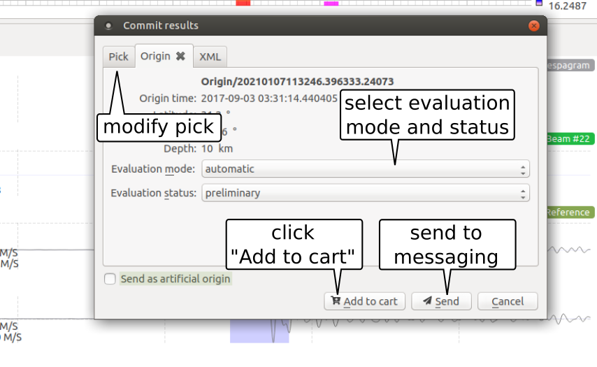
Evaluate and send origin.
Map Widget: View the location grid diagram for evaluating the computed location on the map. For showing the semblance values and the origin location on top of the map in the Map widget, right click on the diagram and choose “Show on map”. You may also save the semblance map to a file.
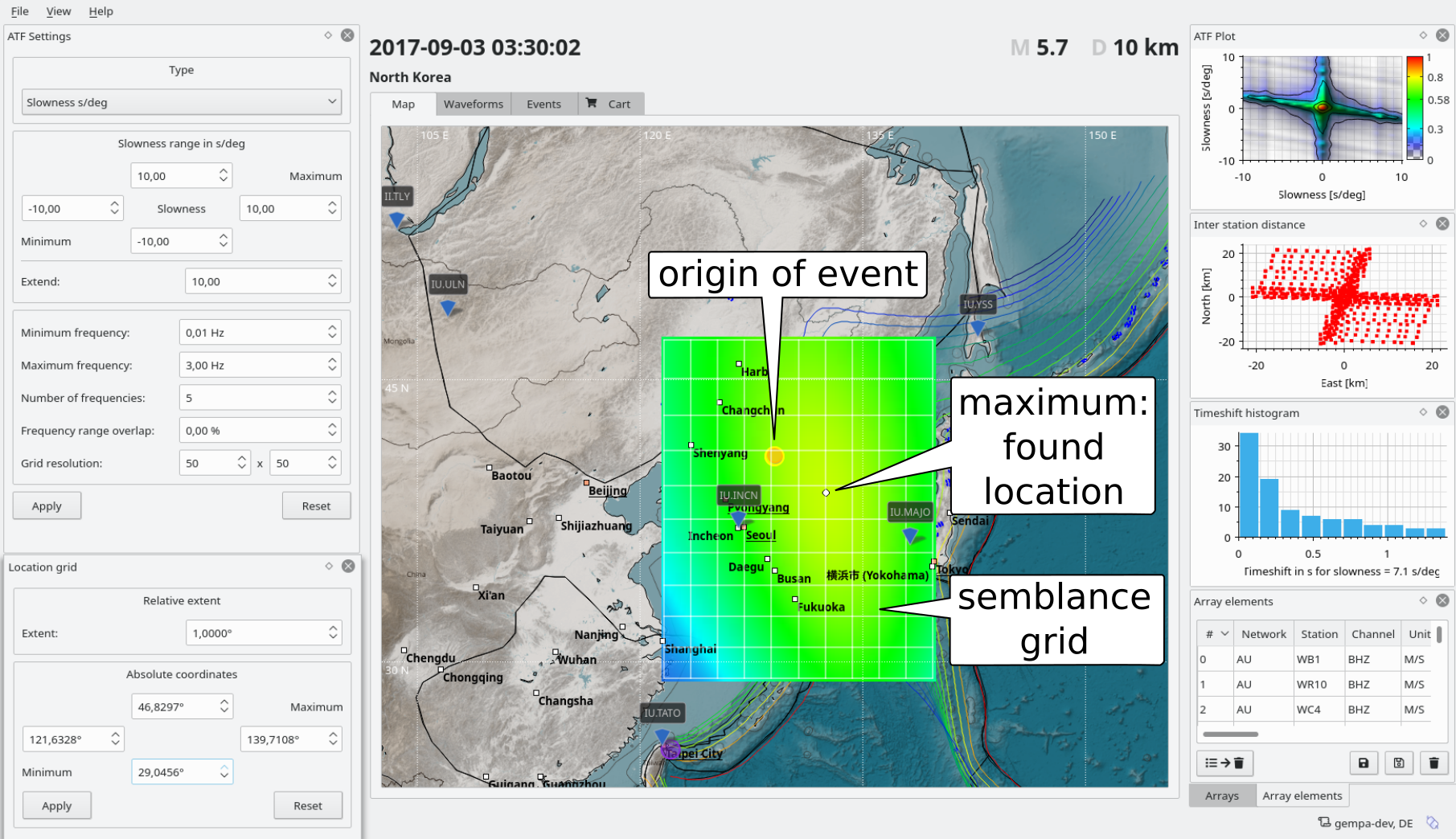
Show semblance grid on map.
Cart widget: After sending the origin parameters are either available in
the cart for further evaluation,
the SeisComP system for further analysis. E.g. adding other picks and for relocating events in scolv. As the beam pick is associated to the reference station of the array it can also be viewed there. The beam pick can be identified by the method B shown along with the pick on the traces.
Phase type identification
not yet implemented
Vespagrams
Vespagrams can be computed based on a selected solution after the slowness-backazimuth, PMCC or backprojection analysis.
Select a solution
For better visibility increase the row height of the vespgram above the traces of the processing widget: Shift + y,
Keep or adjust the backazimuth and the frequency range,
Adjust the vespagram settings:
time window,
slowness range,
Press Update vespagram for computing the vespagram.
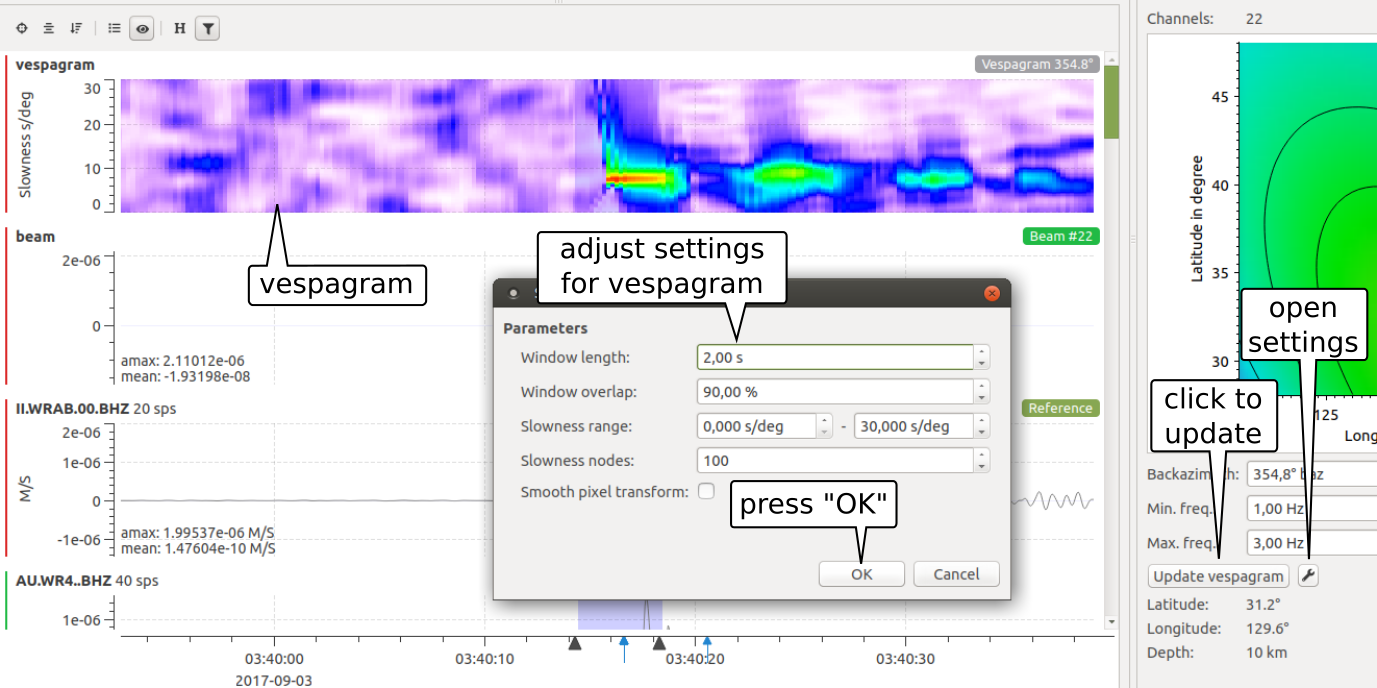
Vespagram based on backazimuth from solution.