Setup and customization
Warning
This section is work in progress and will be subject to future major changes.
Widget arrangement
LAMBDA uses processing and parameter widgets which can be selected or unselected to compose a complete window.
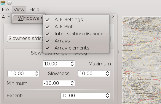
Widget selection for showing in the window.
The widgets can be docked to the window or undocked and used as a separate window. The widgets can also be placed at almost any position within the window. To dock or undock a widget or to change the position click on the widget header and move it to the desired position.
Several widgets can be joined and accessed by clicking on the formed tabs. The size of the widgets be changed by dragging the widget margins.
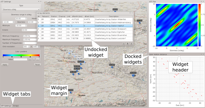
Widget selection for showing in the window.
When LAMBDA is closed the Linux system will save the last widget settings. The system will remember the last widget settings and appy them when opening LAMBDA the next time.
Configuration during runtime
During runtime of LAMBDA some configuration parameters can be overwritten.
General parameters
General parameters such as the data source or the FDSN URL for fetching events. Select Preferences in the File menu and choose Global. The changes will be applied when clicking the Ok button.
Visual parameters
Visual parameters such as color or shading. Select Preferences in the File menu and choose Visual. The changes will be applied when clicking the Ok button.
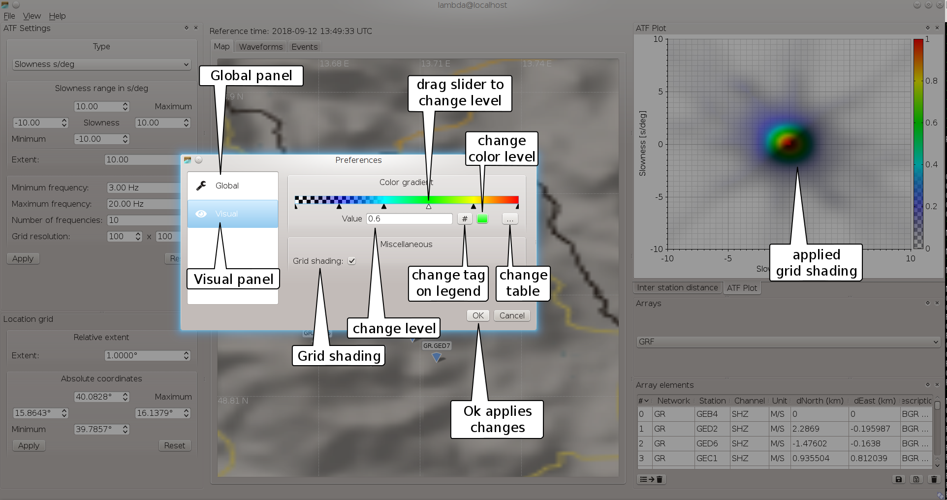
LAMBDA preferences widget with visual parameters.
Array definition
Arrays can be defined by double-clicking on a station symbol on the map for activating or deactivating a station. Station groups can be selected on the map by defining a rectangle on the map. For defining the rectangle hold the shift key and draw the rectangle on the maps by holding the left mouse button pressed. When defining an array the array response function and the inter-station distance plot will update automatically. The array reference station can be selected by selected by double-clicking on the array element in the Array elements window. In the Array elements window array elements can be removed and the arrays configurations can be saved or deleted. When saving, the array configuration will be kept and can also be loaded the next time LAMBDA is started.
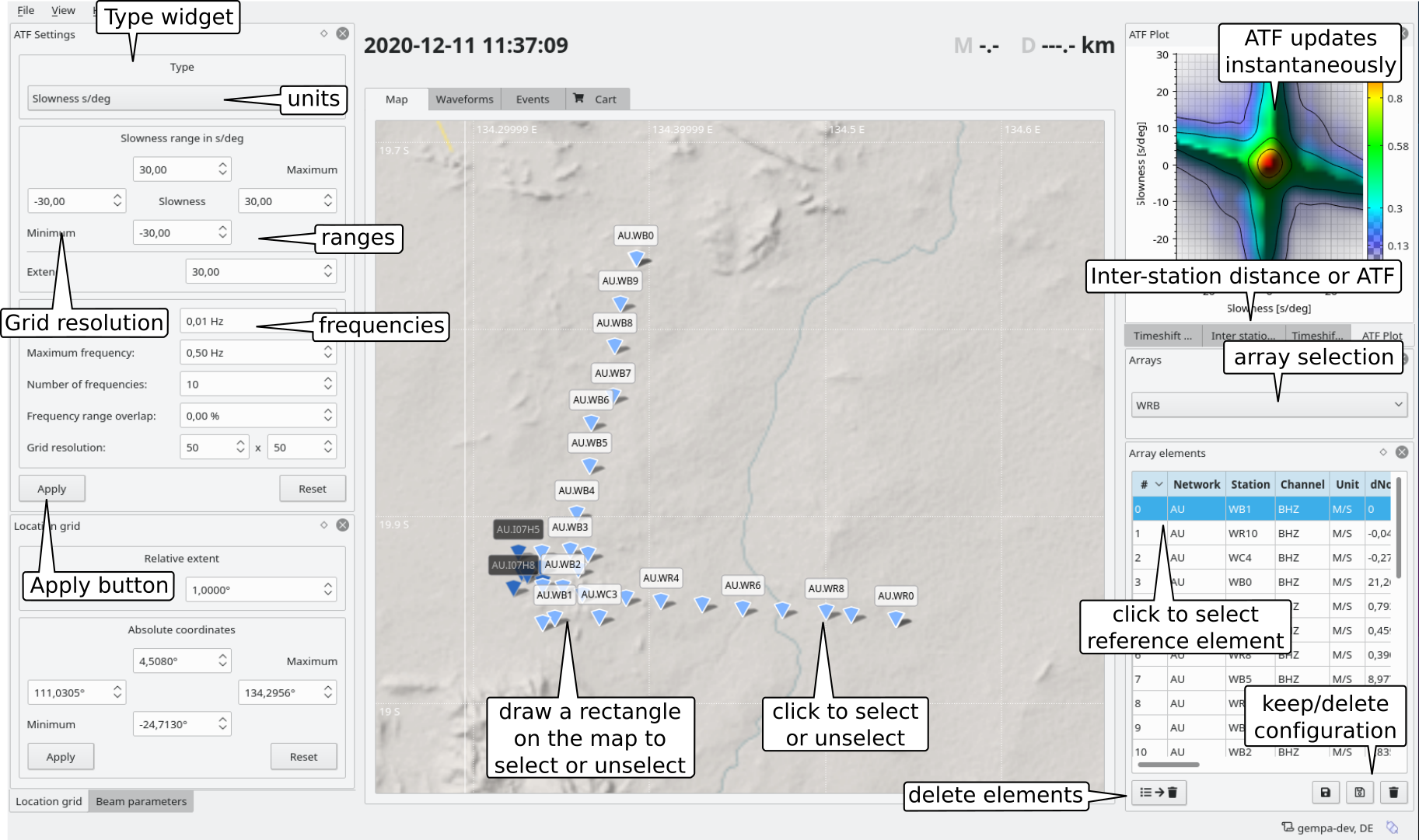
LAMBDA array configuration.
Note
On the map only stations are shown which are which have a valid inventory during the reference time. When starting LAMBDA the reference time is current UTC time. Thus station which were closed before current UTC will initially not appear on the map. However, the reference time can be changed interactively in order to show stations available during the chosen reference time. To change the reference time, right-click on the map and select “Set reference time” from the menu.
Waveform processing and ATF
The data processing and the computation of the ATF can be controlled in the Type widget. Select the units and the range of slowness either as an equal extend from the reference station or separately in N, S, E, and W direction. Set the frequency range, the number of frequency intervals and the grid resolution. Press the Apply button to keep the changes.
Location grid
The location grid that will be used in the back projection method as the search area can defined on the map or in the Location grid widget. Hold the Shift+Ctrl keys and draw a rectangle on the map while holding the left mouse button to make the selection. Select the grid resolution in the Type widget. The parameter can be manually selected in the Location grid widget. To keep the selection, press the apply buttons in the widget where the changes where made.
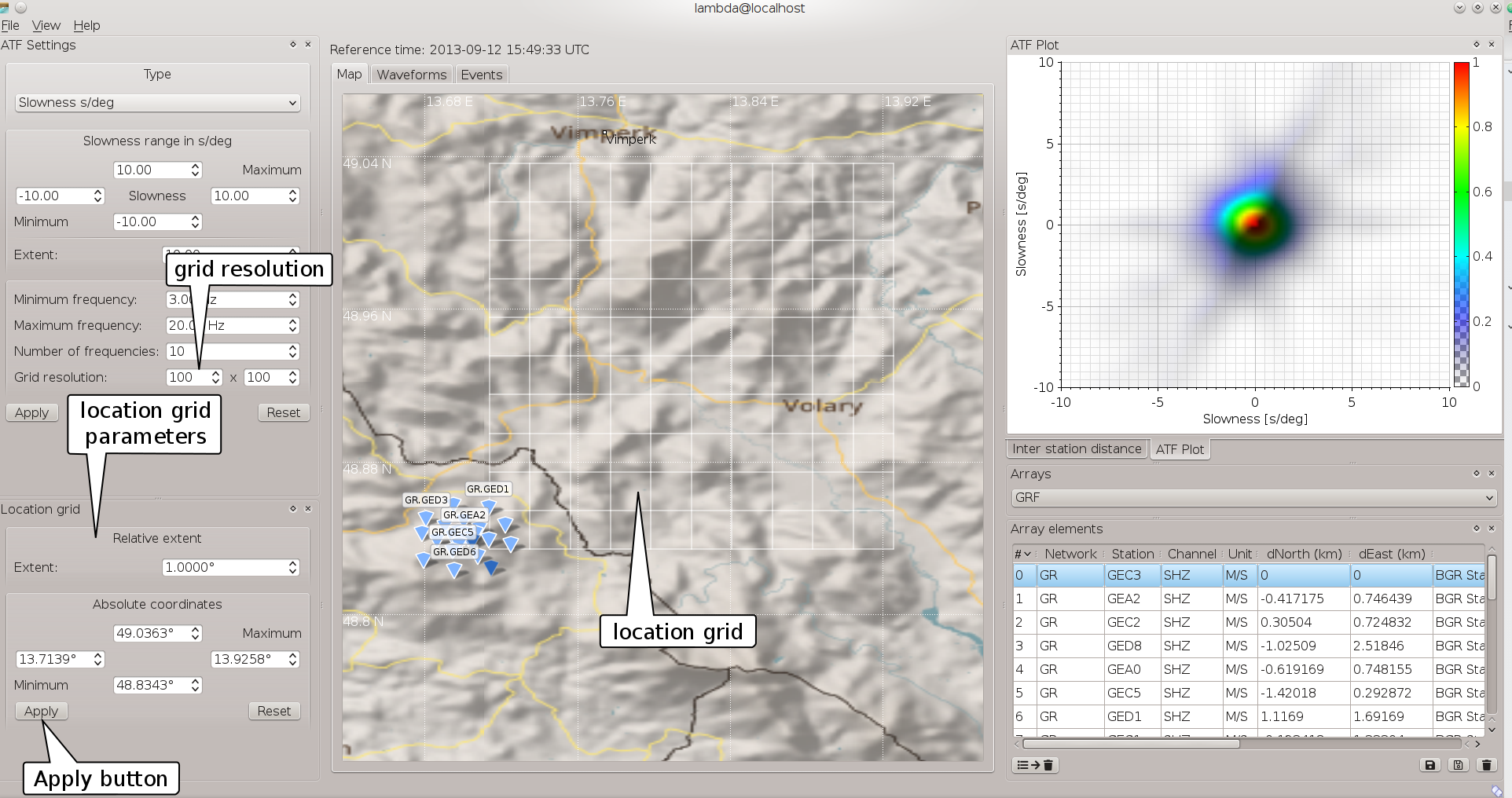
LAMBDA area configuration.
Static configuration
Station information
Import the station inventory using scconfig [10] or manually copy the inventory file in SeisComP XML (SCML) format to SeisComP inventory directory and update the configuration.
cp <inventory-XML file> $SEISCOMP_ROOT/etc/inventory
seiscomp update-config inventory
Array response function (ATF)
The parameters controlling the computation and the visualization of the ATF are set in the configuration file
@SYSTEMCONFIGDIR@/lambda.cfg. Default values and examples can be found in@SYSTEMCONFIGDIR@/defaults/lambda.cfg.Type and unit of input values, possible values are: s/km, s/deg:
atf.unit = s/deg
Frequencies (applicable only when considering units of slowness, not wavenumber) for input values
atf.minFrequency = 1
atf.maxFrequency = 10
atf.frequencySteps = 10
Ranges of input values in units of atf.unit:
atf.minRangeX = -50
atf.minRangeY = -50
atf.maxRangeX = 50
atf.maxRangeY = 50
Number of grid intervals:
atf.grid.x = 101
atf.grid.y = 101
Color definition of ATF and array analysis in a list of comma-separated tuples of semblance:color code. The color code is given in hexadecimal representation. The transparency given by the alpha value may be added, e.g.:
atf.gradient = 0:00000000,0.2:0000ff80,0.4:00ffff,0.6:00ff00,0.8:ffff00,1:ff0000
Array definition
Defining the array seems simple, at first hand. Obviously stations as array elements need to be defined. However, since stations and event networks are subject frequent changes due to maintenance, re-configuration, re-location, etc. epochs of constant configuration need to be considered. On the other hand, possible changes should be allowed to avoid that array configurations become obsolete when location codes change or data logger are exchanged. Therefore, one comma-separated list of network.station.location.channel is defined per array defining the array elements.
Example for the definition of the Graefenberg array, GRF, in Germany:
arrays = GRF
arrays.GRF.channels = GR.GRA1..HHZ,GR.GRA2..HHZ,GR.GRA3..HHZ,GR.GRA4..HHZ,GR.GRB1..HHZ,GR.GRB2..HHZ,GR.GRB3..HHZ,GR.GRB4..HHZ,GR.GRB5..HHZ,GR.GRC1..HHZ,GR.GRC2..HHZ,GR.GRC2..HHZ,GR.GRC4..HHZ
In addition alternative values can be given for each value. The alternatives are given separated by colon
`:`. The fist value in the list of alternatives takes priority. When the channel with the prioritized value is not available at the considered time, the next value is chosen. In this way, the most appropriate channel is chosen.example for allowing location codes [..,.10,20,30] and channels code [HHZ, BHZ] to be considered for station PB02 of the CX network,
CX.PB02.:10:20:30.HHZ:BHZ
or alternative stations [PB02,PB03], e.g.:
CX.PB02..HHZ:CX.PB03..HHZ
or for a full configuration of stations from the CX and the 4A networks forming two separate arrays, A and 4A, respectively:
arrays = A,4A
arrays.A.channels = CX.PB01.:00.HHZ, CX.PB02.:10:20:30.HHZ.HHZ:BHZ, CX.PB03..HHZ, CX.PB04..HHZ
arrays.4A.channels = 4A.CSA0.01.HHZ, 4A.CSA1.01.HHZ, 4A.CSA2.01.HHZ, 4A.CSA3.01.HHZ, 4A.CSA4.01.HHZ, 4A.CSA5.01.HHZ
The array names are use and referred to in lambda and autolambda.