SIGMA: Interactive Processing

Interactive ground motion processing is provided by SIGMA. SIGMA may be invoked on the commandline e.g. with informative debug output:

$ seiscomp exec sigma --debug

Workflow recipes

The workflow recipes can be followed from the beginning to the end for using SIGMA to analyze ground motion parameters for events in SIGMA. The recipes can also be used in bits and pieces to exercise particular tasks.

Event or Incident import

First the event or the incident which is to be processed must be loaded. Import an event from the SeisComP database or from a FDSNWS provider by selecting Import events. Import an incident by clicking on the incident in the list of incidents.

When searching for events or incidents, filter options are available for selecting in the events according to time, region, magnitude and depth.

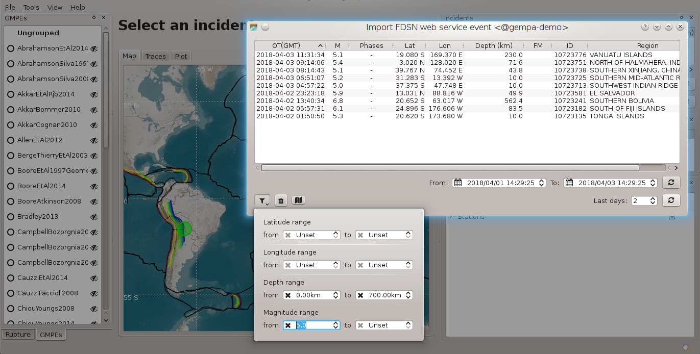
Figure 37: Event selection using FDSNWS and filter options.

Defining rupture parameters

The focal mechanism and a rupture geometry may be required depending on the considered GMPEs/GMMs. The section GMPE/GMM: Ground Motion Prediction Equations and Models provides the detailed information.

The focal mechanism is either

• provided by the event and may be adjusted or

• set interactively in SIGMA

to match geological knowledge.

The rupture geometry can be defined interactively in SIGMA based on a focal mechanism which

• pre-defined or

• entered in the Rupture widget.

For adjusting the focal mechanism enter the 3 angles, strike, dip and rake, or drag the beach ball:

1. Chose Edit focal mechanism in the Tools menu of SIGMA,

2. Click on the focal mechanism to drag it or change the tabulated values to the desired value,

3. Click on a radio button to define the fault plane out of the two nodal planes,

4. Click the OK button to use the values within SIGMA.

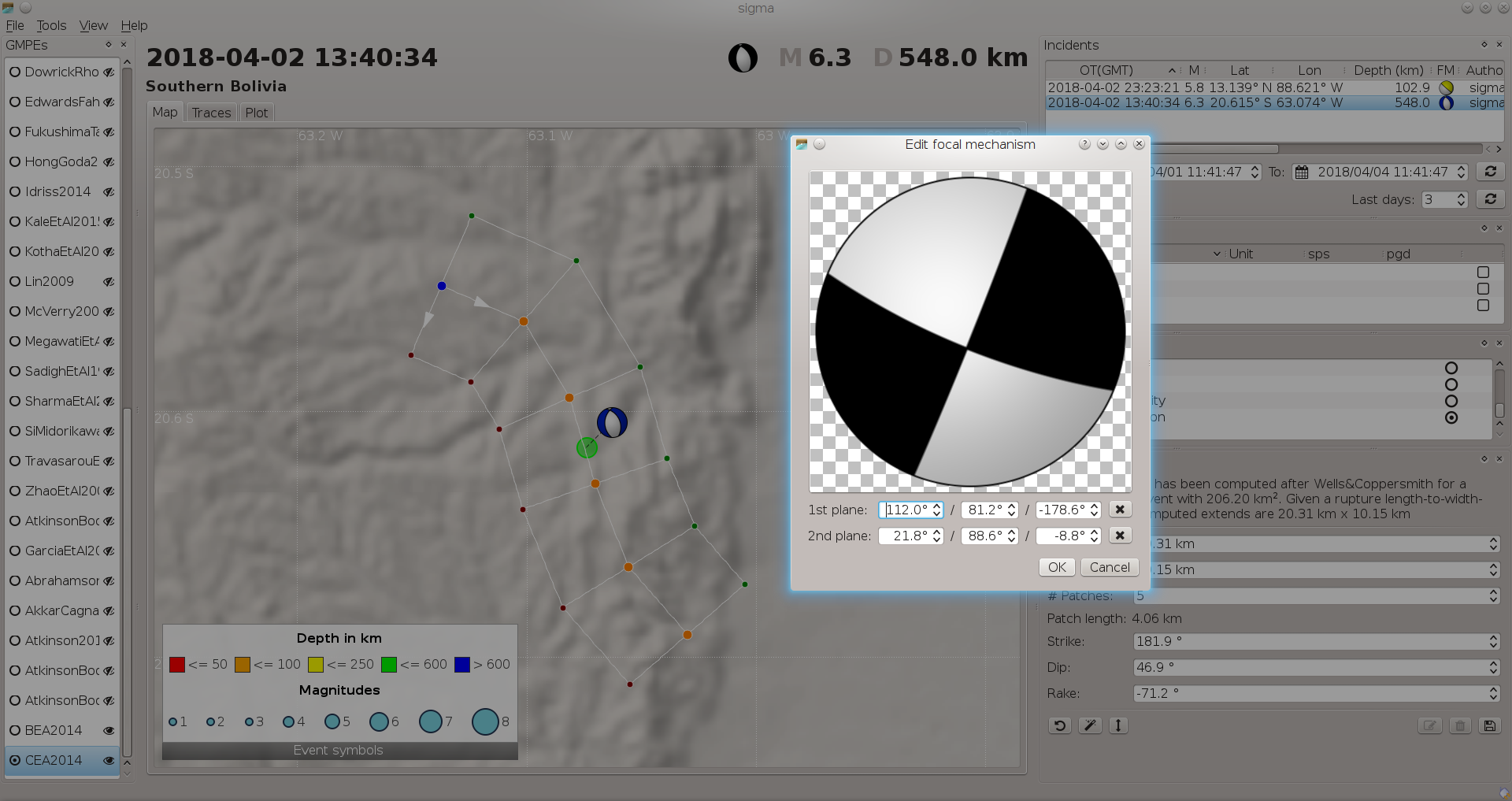
Figure 38: Adjust the focal mechanism by dragging the stereographic projection.

For defining the rupture geometry

1. Choose the Rupture widget in the View menu,

2. Enter the desired values, Length, Width and # Patches for defining the rupture geometry,

3. Accept an existing focal mechanism or enter strike, dip and rake to set a new one,

4. Click on the magic wand to generate the rupture based on the changes. The geometry may be adjusted by dragging the ruputre on the map, e.g. to match a known fault. When the rupture is defined by more than one patch then each patch can be dragged individually typically impacting the geometry of all other patches. Dragging the rupture will modify the strike angle by keeping the dip and the rake constant.

5. When satisfied with the geometry press the save button in the lower right to accept the parameters.

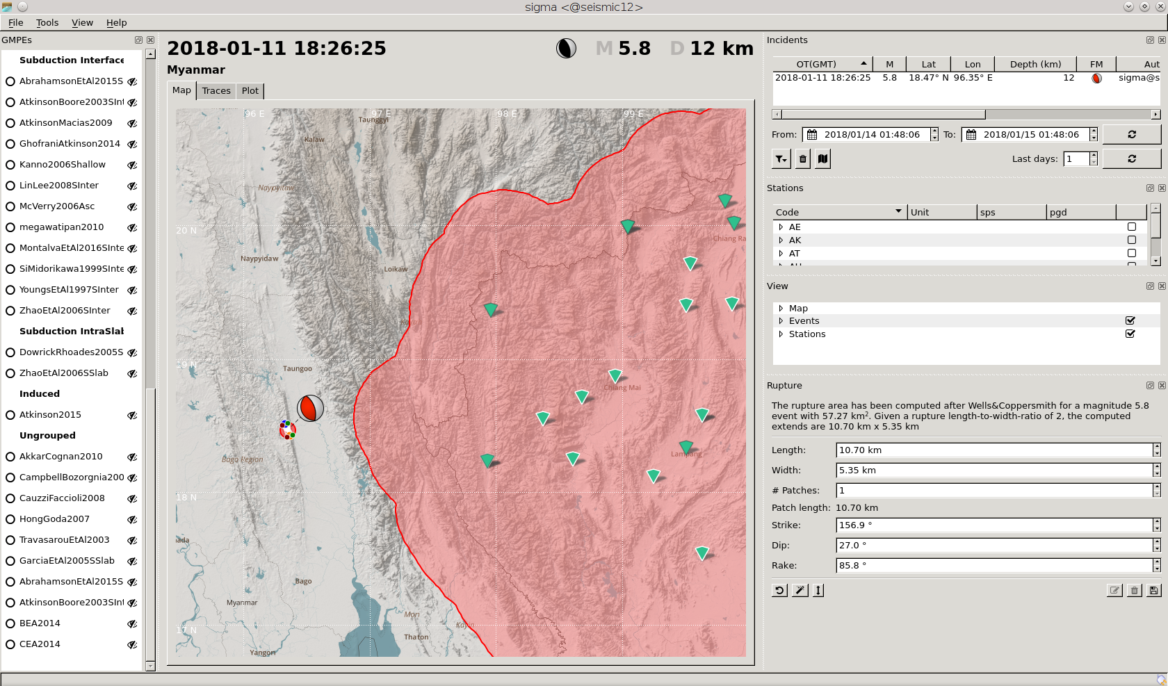
Figure 39: Adjust the rupture parameters by value in the Rupture widget.

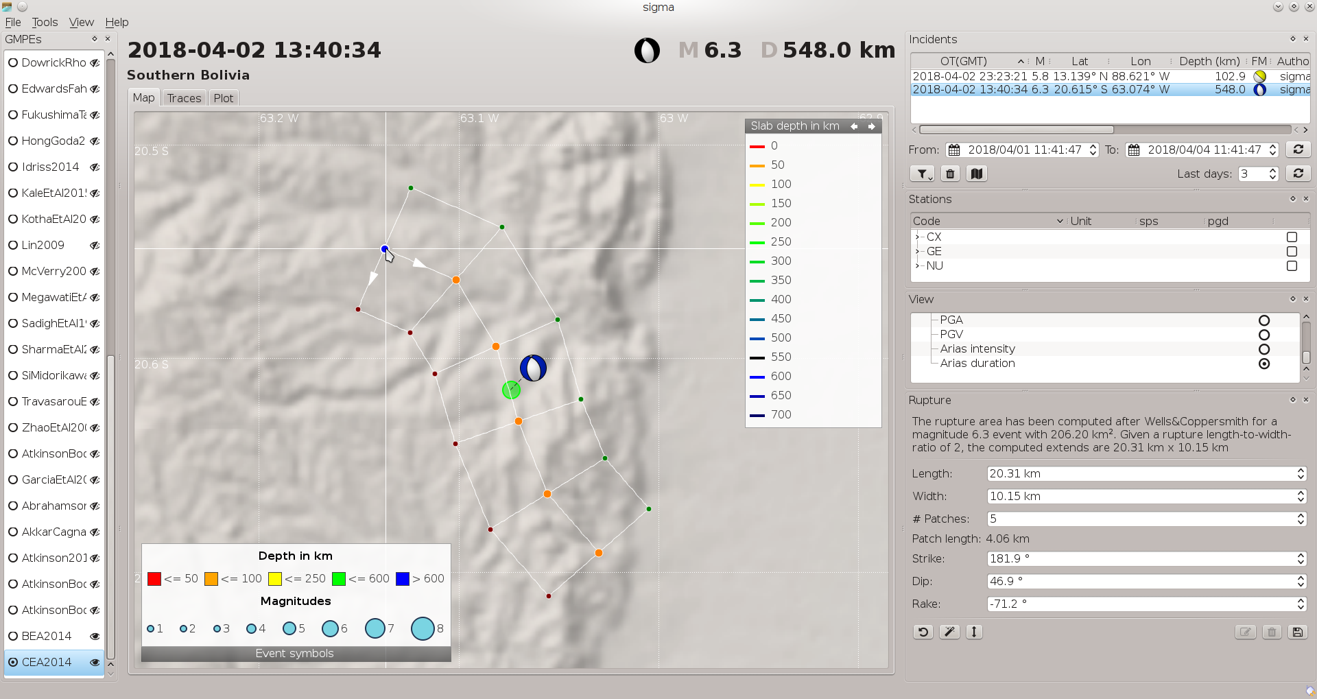
Figure 40: Adjust the rupture by dragging the surface projection of the rupture.

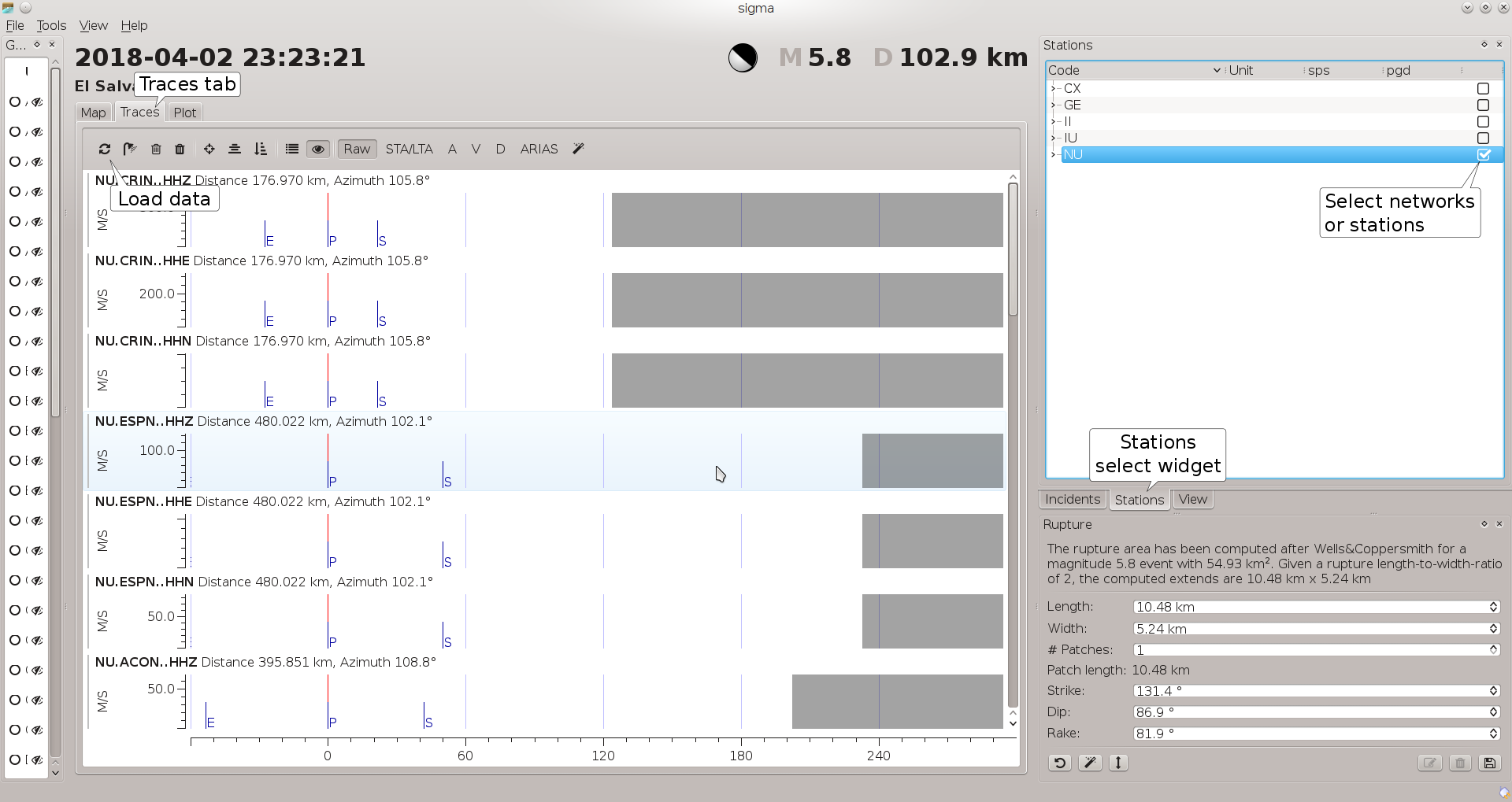
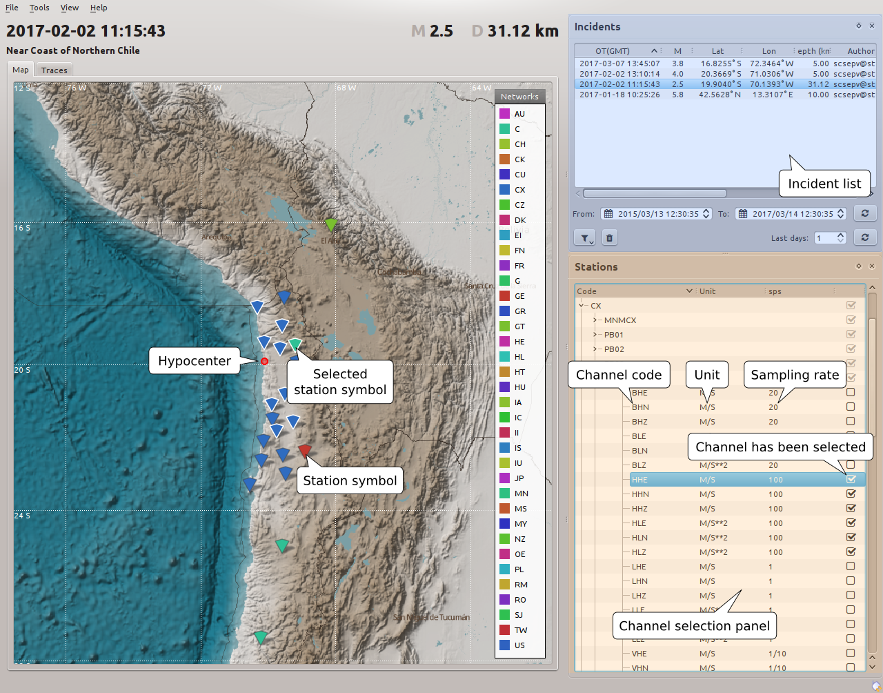
Data selection

Predicted values can be compared with actually measured data. In order to load the data select the stations in the Stations window and click on the Load data button which can be found in the Traces tab.

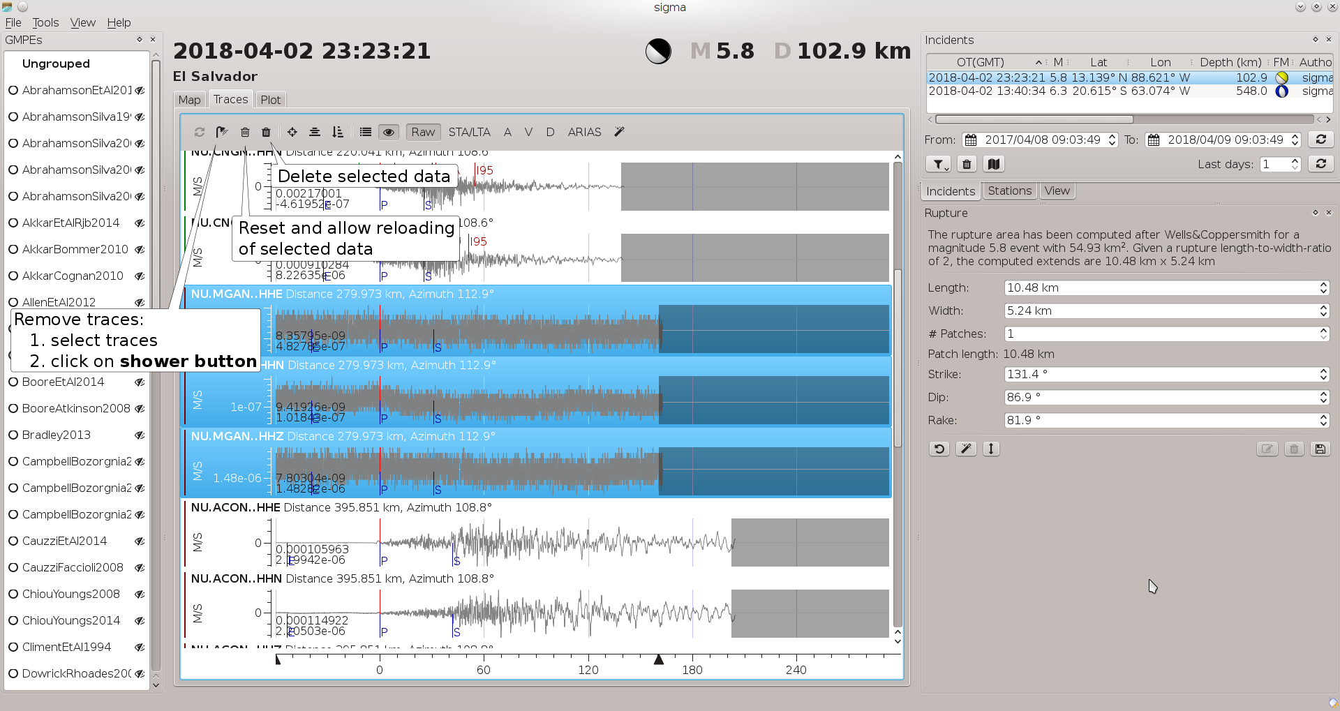
Empty traces will disappear after pressing the shower button. If data are unusable or traces should be deactivated or removed for another reason, select a trace by clicking on it. Clicking on the trash cans deletes the traces. Clicking on the gray trash can also allows to reload the data.

Note

Several traces can be multi-selected using the Control or the Shift key while clicking on several traces.

By default, traces are sorted by network and station name. For sorting by epicentral distance click on the sort button.

Data processing

Because multiple channels with different instruments and different sample rates can be acquired per station, SIGMA will select the default set of channels with the following AUTOSIGMA:

• Read the bindings variable channels and select all channels that either match the full string or the string without the last character (component code). E.g. if BH is configured, it will match BHZ, BHN and BHE. If BHZ is configured, it will only match BHZ. Furthermore only channels with unit m/s or m/s**2 will be taken into account.

• If channels is not defined then SIGMA will select velocity and strong motion channels with the highest sampling rates. Again, only channels with unit m/s or m/s**2 will be taken into account.

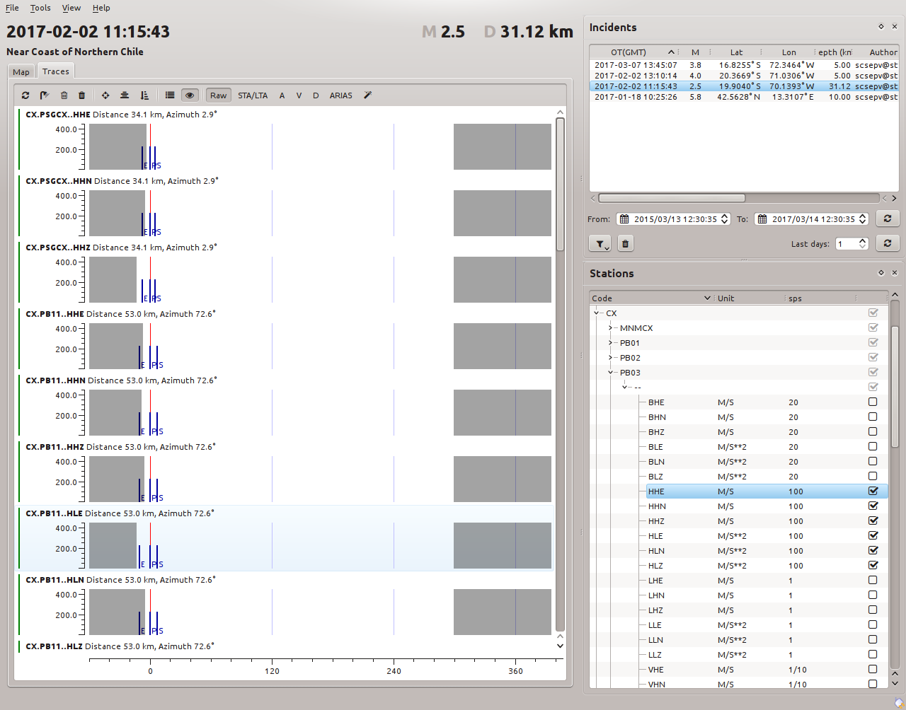
Each channel selection can be changed interactively in the inventory tree panel. This will automatically add a trace row in the Traces Window. Each activated channel corresponds to a row of the trace list. That list holds all potential candidates for processing.

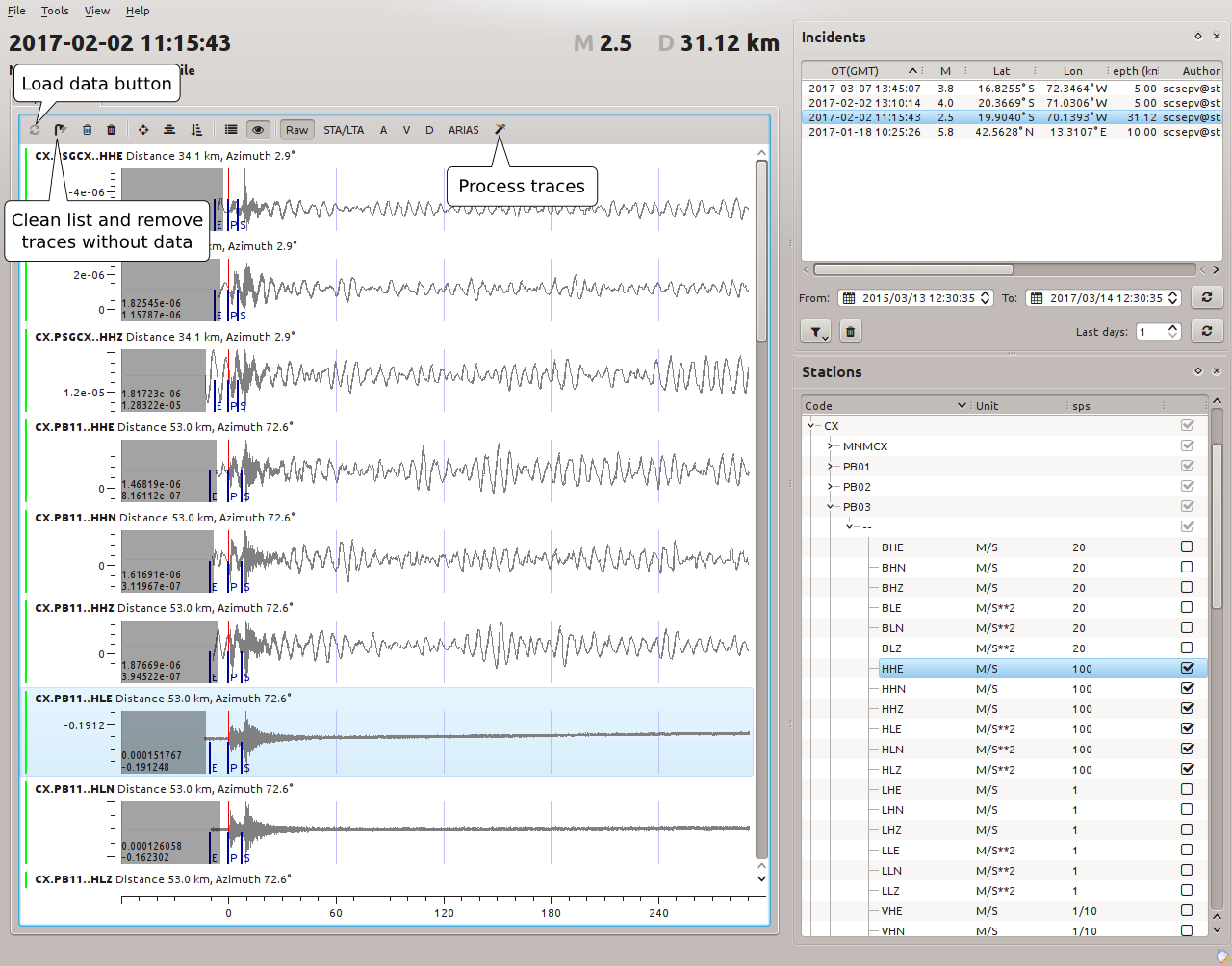
Before processing can be done, the data must be loaded. Once the list is (almost) completely configured, the load button has to be used to load data for all empty traces. During loading all color indicators (left hand border) for traces that are currently loading turn to yellow. Once a trace is complete the color turns into green. If data is incomplete or missing at all then it turns into red. Light colors are used for data acquisition results.

The default time window to load data for is [-60s; 300s] around the P onset. This time window can be changed with processing.preEventWindowLength and processing.postEventWindowLength.

The time window can be changed interactively by selecting a trace and by moving the triangle handles on the ruler.

Once the data have been loaded, the default data processing can be started by clicking on the magic wand. The calculated values are shown on the traces. The color bars to the left of the traces indicate success or possible issues. Switching between processed data including STA/LTA, acceleration, velocity, displacement and arias intensity is provided. The Default data processing including filtering can be modified in the Preferences window.

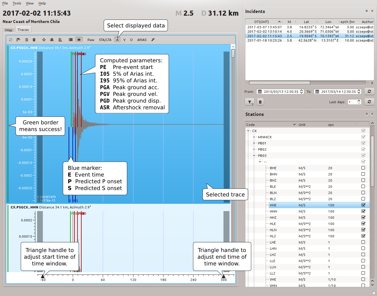
Figure 45: Calculated parameters

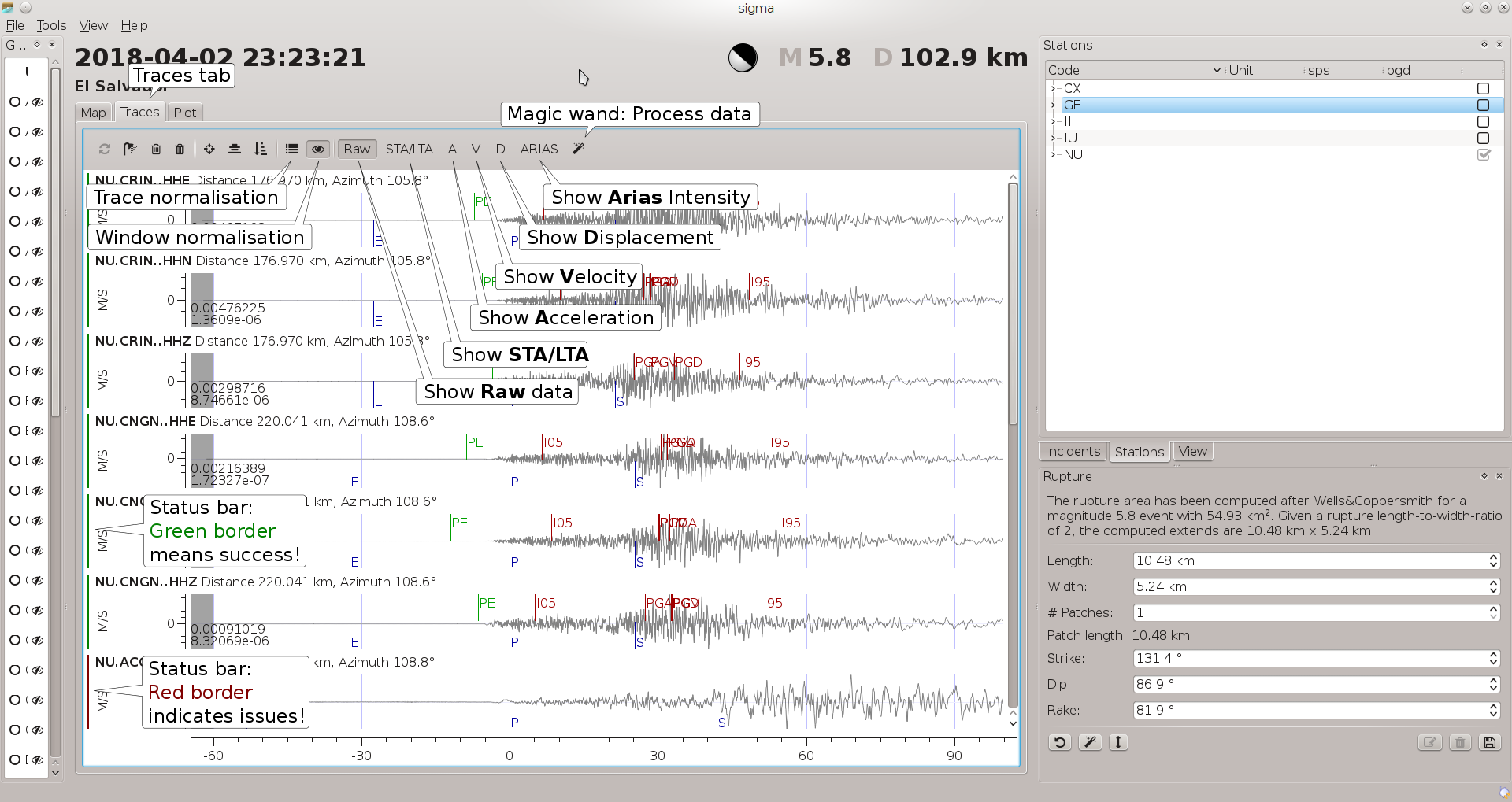
Figure 46: Switch buttons to show different trace quantities

Trace markers

The trace markers in the time where the respective quantities are calculated.

Marker	Description
PE	Processing start time - beginning of computed pre event window.
I05	5% of Arias intensity.
I95	95% of Arias intensity.
PGA	Time of the peak ground acceleration measure.
PGV	Time of the peak ground velocity measure.
PGD	Time of the peak ground displacement measure.
ASR	Aftershock removal detection marker.

Algorithms and parameters

Processing is done for each trace separately. The following parameters will be computed:

• Arias intensity

• 5% and 95% of Arias intensity

• Duration

• Characteristic intensity

• Effective Design Acceleration

• Specific Energy Density

• Cumulative Absolute Velocity

• Predominant period

• Mean Period

• Peak ground acceleration

• Peak ground velocity

• Peak ground displacement

• Pseudo acceleration response spectra

The following steps are performed to compute the parameters:

1. Trim data

   The input data is trimmed to match exactly the requested processing time window. Because a trace is a list of records and each record covers a certain time range, it is not very likely that the requested time window start time or end time falls on a record border.

2. Gain correction

   The input is the raw data of the sensor in COUNTS, so the this processing step applies the gain to the data to convert the COUNTS to the sensor unit: meters per second or meters per second squared.

3. Demean

   The arithmetic mean of all samples is computed and subtracted from each sample.

4. Differentiate (velocity only)

   If input data is velocity then differentiate it to acceleration.

5. Spectrum computation

   The spectrum computation copies the current data and applies several processing steps on them. E.g. the taper and zero padding are not applied to the data used in the next step.

   1. Taper

      Apply the configured window function to the data with configured length at either side. The default window function is the Hann window [3].

   2. Zero padding

      Pad the data on either side with zeros. The number of zeros depends on processing.spectra.padLength. If that value is negative then the pad length in seconds is determined from 1.5 * processing.filter.order / processing.filter.loFreq.

   3. FFT

      Compute the spectrum of the data with fft.

6. STA/LTA check

   If processing.STALTAratio is a non-zero positive number then the STA/LTA function is computed. The STA length is the minimum of processing.STAlength and processing.preEventWindowLength. The LTA length is the minimum of processing.LTAlength and the available data window prior to trigger time. The threshold is checked either on the entire STA/LTA trace or only around the trigger time with a configured margin. This margin must be non-zero positive number to be taken into account. If the threshold is not exceeded then the further trace processing is discarded.

7. Pre-event cut-off

   If pre event cut-off is enabled then a hardcoded STA/LTA algorithm (with STA = 0.1 s, LTA = 2 s, STA/LTA threshold = 1.2) is run on the time window defined by (trigger - 15 s). The pre event window is hence defined as [t(STA/LTA = 1.2) - 15.5 s, t(STA/LTA = 1.2) - 0.5 s]. The data before the pre-event window are trimmed.

   Otherwise the pre-event window is defined between the first data sample and the trigger time.

8. Pre-event offset

   Compute the mean of the pre-event window and removes it from the entire trace.

9. Detrend

   Compute the global linear trend and correct for it.

10. Aftershock removal

    If enabled then the curvature of the second derivative of relative Arias intensity is checked to detect aftershocks and to trim the signal window.

11. Filtering An causal filter is applied with configured parameters.

12. Integrate to velocity and displacement

    Integrate the data to achieve ground velocity or displacement.

13. Compute parameters

For detailed processing of individual traces, click on the trace data. This will open a new interactive processing window in which the processing parameters as well as the input parameters can be changed. To apply the modified parameters click Reprocess.

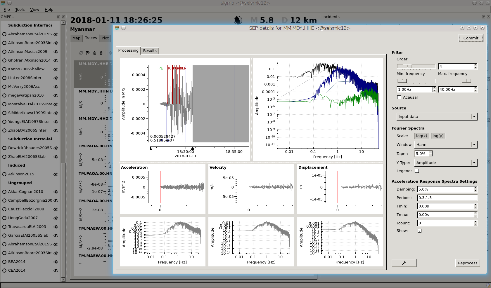
Figure 47: Processing window

The new window also has a Results tab in which the results values can be viewed. Click on Commit when the processing is finished to keep the modified values in SIGMA. Thereafter, processing the next trace can be started.

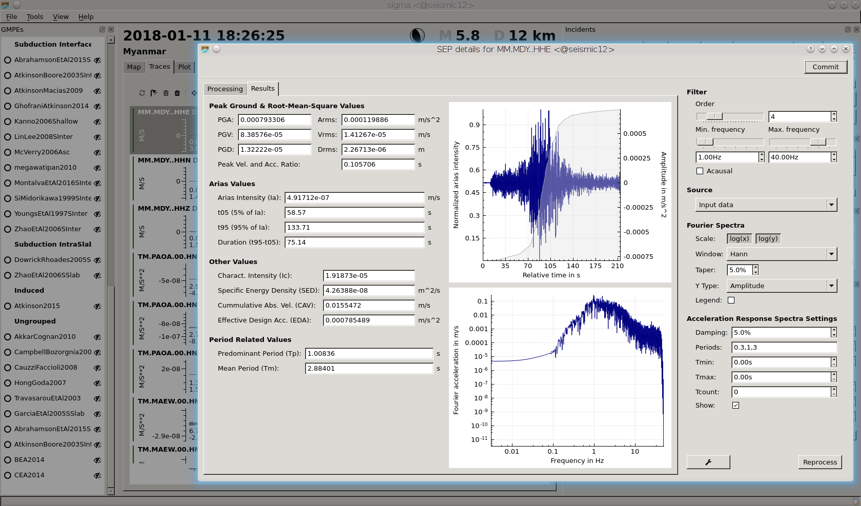
Figure 48: Result window

Note

In order to store the processing results, they must be saved as an incident in the configured database. Committing alone only keeps the parameters in the RAM. If not stored in the database, they will be lost after closing SIGMA.

Shake maps and parameters on map

Select the Map perspective to view predictions from GMPEs/GMMs or parameters measured from waveoforms. For viewing predictions select the GMPE to be considered in the GMPEs widget and one of the value to be shown in the View widget. The vizualized values calculated from GMPEs/GMMs are:

• MMI

• GMPE (PGA): PGA

• GMPE (PGS 0.3s): Pseudo Spectral Amplitude measured at 0.3 s period

• GMPE (PGS 1.0s): Pseudo Spectral Amplitude measured at 1.0 s period

• GMPE (PGS 3.0s): Pseudo Spectral Amplitude measured at 3.0 s period

• GMPE (PGV): PGV

When the respective value has been measured on waveforms from the station it is also shown at the station allowing a direct comparison. Otherwise the station symbol takes the color corresponding to the predicted value.

To show some of the parameters measured from waveforms select among:

• PGA

• PGV

• Arias intensity, Ia

• Arias duration

The color scaling is adjusted automatically.

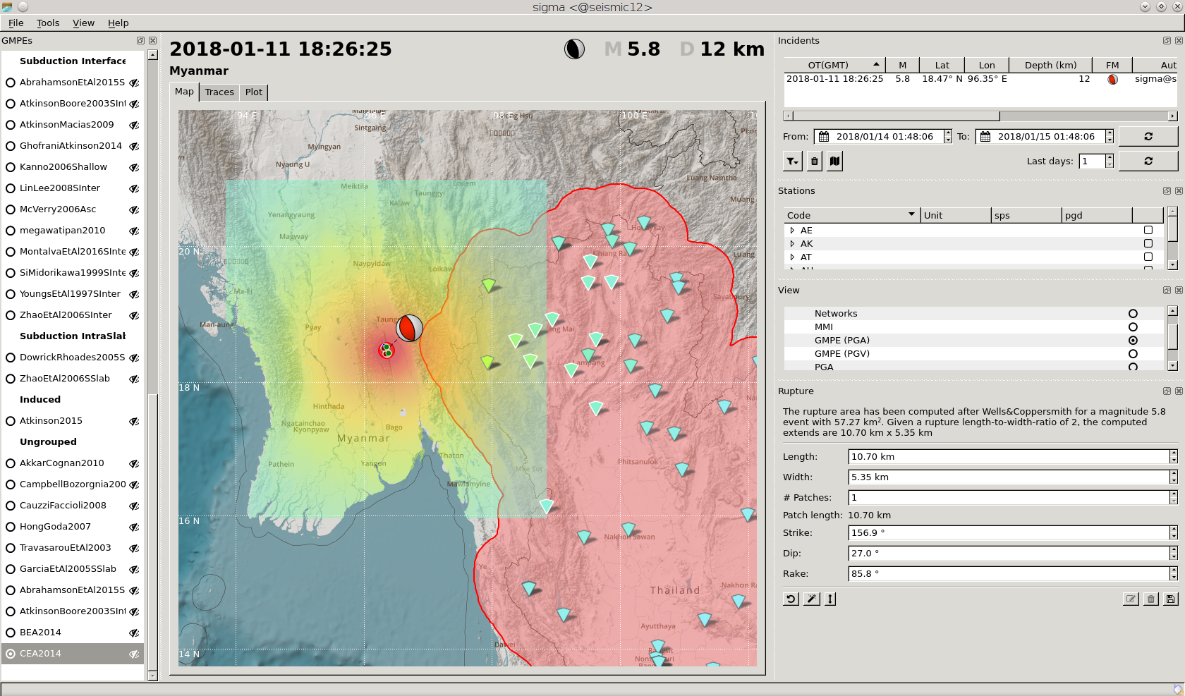
Figure 49: Predicted PGA shwon in the map window.

Select map features such as colouring, contours etc. in the Map section of the View window. Legends are activated/deactivated in the View menu or by right-clicking on a map.

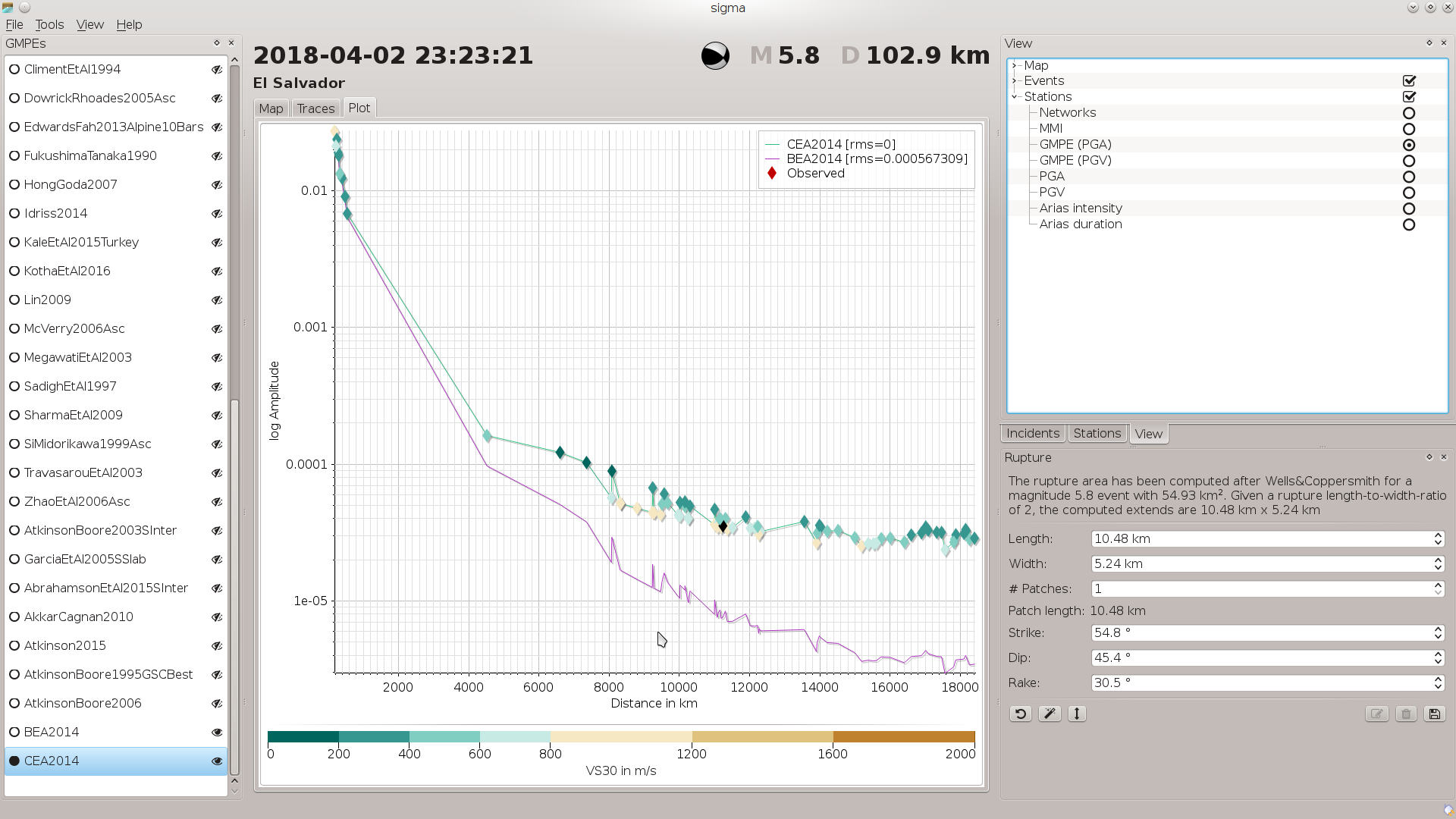
GMPE plots

For plotting predicted ground motion parameter alongside measured and derived values choose the preferred GMPE in the GMPEs window. The eye symbol to the left of the GMPE indicates which GMPE is activated for viewing. The GMPEs and the data values will be shown in the Plot tab.

To actually evaluate the ground motion parameters in the Plot tab choose a GMPE in the GMPEs window and a valid parameter in the View window. This will command SIGMA to calculate the parameter values. The rms value in the legend refers to the rms residual of the values calculated based on the indicated GMPE model the reference GMPE. The reference GMPE is the selected by clicking in the circle field to the left of the name of the GMPE in the GMPEs window. When selecting GMPE, the boxes shown in the Plot tab indicate values predicted for stations.

Note

Which ground motion parameters can be calculated, depends on the selected GMPE. The GMPEs “BEA2014” and “CEA2014” provide the complete set of parameters.

Predicted ground motion parameters can be compared with values measured at the stations by selecting all other parameters than “GMPE” in the View window. In this case, the rms value in the legend shows the difference between the predictions and the measured values. The maximum distance of involved stations depends on the configured distance and the configured maximum signal-to-noise ratio.

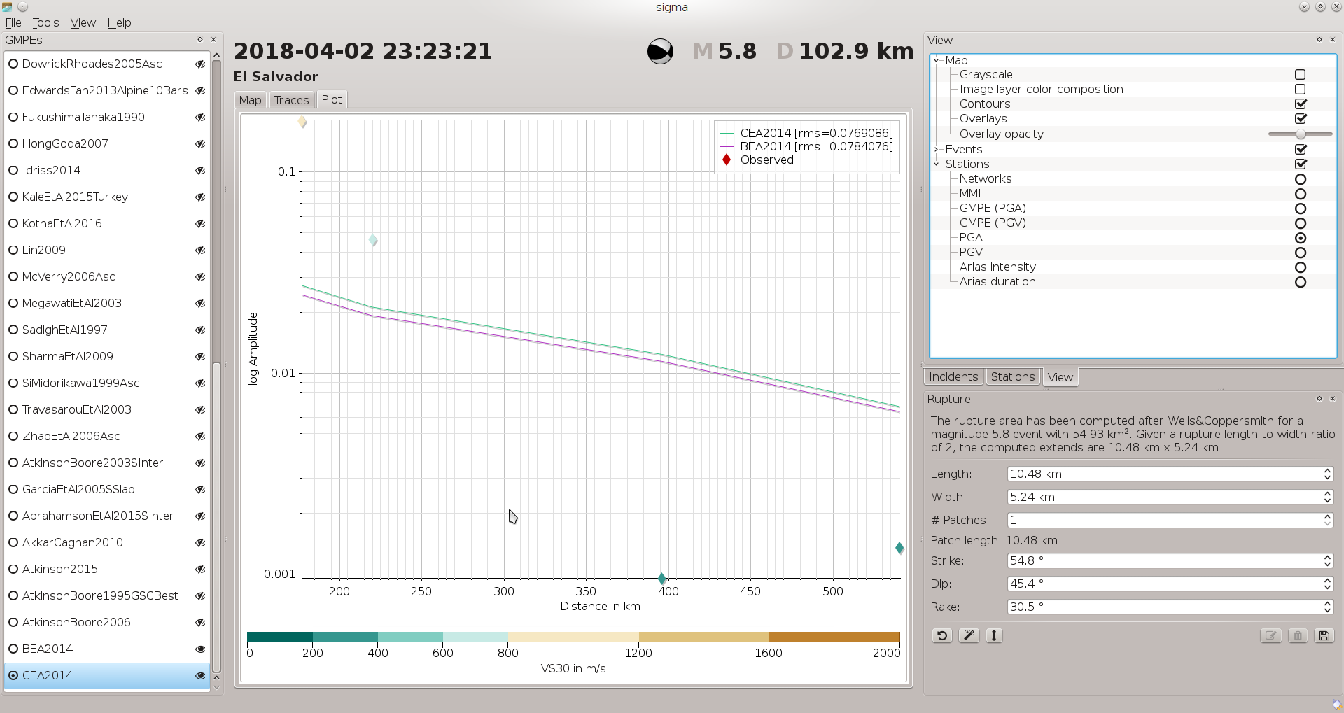
Note

While “GMPE” in the View window refers to the values predicted based on the selected GMPEs, all other options refer to values actually measured at the station. Values at grid points without station values are always predictions.

GMPE comparison

GMPEs are typically valid for a particular region or for a particular set of data. In SIGMA they can be compared and the most appropriate GMPE can be identified.

1. In the GEMPEs window select the GMPEs which should be analyzed by clicking on the eye symbol. When the eye symbole is striked through, then the GMPE is not selected.

2. In the View window select the PGA or PGV to compare the GMPEs with measured the data.

3. Open the Plot window and compare the values measured at the stations with the predictions. The rms value in the legend indicates the rms residual between the GMPE and the measured data. The best matching GMPE can be identified for future processing.

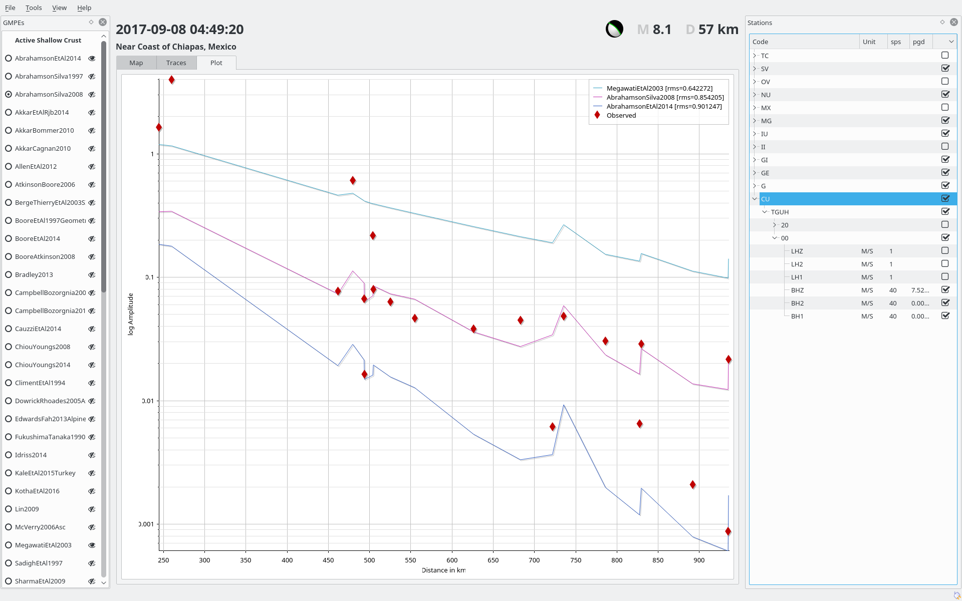
Figure 52: GMPE comparison with measured data

Saving incidents

Store the processing results as an incident in the SIGMA database in order to keep the results. Otherwise the calculated parameters will be lost. To save the incidents, open the Save incidents dialog in the File menu. The saved incidents can be read and opened using the Incidents window.

Generate screenshots

Save map images to PNG files like screenshots using the File menu.

Export incidents and generate reports

Incidents can be exported and reports can be generated based on customized scripts. The scripts can take selectable input parameters. They must be provided by the operator. To invoke the export and report generation select the Export incident dialog in the File menu. Choose the output directory and the customized script along with the TODO options.

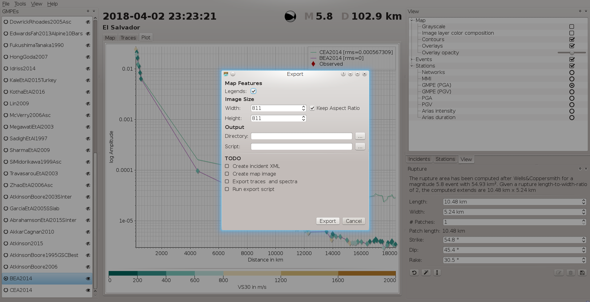
Figure 53: Export incident.

Read the documentation on the configuration of reports for details on customization.

Incidents

The data processing is triggered by and internal incidents are based on existing events. From events SIGMA extracts the important parameters such as source and magnitude and creates the internal incidents. The internal incident can be stored into the SIGMA database. SIGMA will select all stations within processing.maximumEpicentralDistance kilometers with respect to the hypocenter. To avoid processing of redundant channels (e.g. decimated channels) or channels that do not record ground motion (e.g. temperature), SIGMA selects a set of channels for each station which will be processed if data are available.

The list of incidents is by default located at the upper right area.

Customization by configuration

The calculations can be customized within SIGMA. To make permanent changes adjust the configuration parameter using scconfig [10]. Restart SIGMA to make use of the changes.

seiscomp exec sigma

On-the-fly customization

General and processing parameters defined by the configuration can be adjusted by the user within SIGMA using the Preferences dialog of the File menu. The changes will be applied on-the-fly. The applied parameter changes are only available while SIGMA is executed. Any change will be lost after SIGMA is closed.

Widget re-arrangement

The SIGMA GUIs is composed of several windows (widgets). The widgets show parameters in tables, diagrams or maps or allow interactive control of the data processing. Click on the widget header on the top of each widget and drag the widget using the mouse in order to re-arrange the widget.

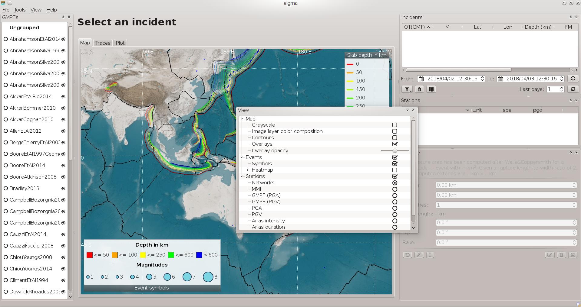
Figure 55: Place a widget by dragging with the mouse.

Widgets may be chosen to be hidden or made visable by selecting the respective window in the Windows section of the View menu of SIGMA.

Data, database, FDSNWS, units, colors

General parameters can be set in SIGMA by the operator. To access the parameters open the Preferences dialog in the File menu of SIGMA and choose the Global section. The changes are immediately available when pressing OK.

The parameters that can be adjusted include:

• source of waveform data

• the SIGMA database

• the FDSNWS for fetching event parameters

• units

• colors of gradients and heat maps

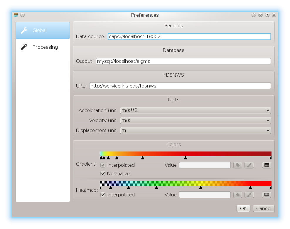
Figure 56: Global preferences

Processing parameters

Parameters controlling the data processing and prediction can be adjusted in SIGMA. To access the parameters open the Preferences dialog in the File menu of SIGMA and choose the Processing section. The changes are immediately available when pressing OK.

The parameters that can be adjusted include:

• Maximum epicentral distance of stations to be considered

• Area around the epicentre considered when applying the GMPEs and pixel resolution

• Time windowing and processing of waveforms

• Calculation of Fourier spectra

• Calculation of Response spectra

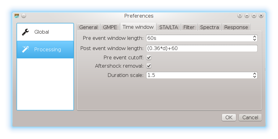
Figure 57: Processing preferences