Algorithms
scautomt and scmtv invert processed waveforms from multiple
seismic phases for seismic moment tensors in the time
domain. Either the deviatoric or the full moment tensor can
be computed as controlled by automt.invertFor6Components. Inversion
for deviatoric and full moment tensors require 8 and 10 component
Green’s functions, respectively.
For inversion the full response information including those for the sensor and the data logger must be available. They can be generated by SMP [1].
Data processing and inversion
The data processing is pre-configured by magnitude-dependent profiles. Each profiles defined the seismic phases to be considered along with the component, time windows, period (hence frequency) range, minimum SNR, weighting, etc. After choosing the profile, the data processing and inversion works as follows:
Acquire waveform data of all three components of configured stations with respect to P onset and the configured signal length (see section Time windows) including a configurable margin and a epicentral distance range (
automt.profiles.$name.minDist-automt.maximumDistance).Restitute data to displacement
Load Green’s functions for each station
The data is resampled at the sampling frequency of the Green’s functions.
Rotate 3 components into ZRT system
Extract configured time windows and apply bandpass-filtering
Align waveform data with Green’s functions by cross correlation to obtain the best phase match. The maximum shift allowed for the entire dataset is given by
automt.profiles.$name.maxShiftin steps ofautomt.profiles.$name.shiftStepto account for differences of the centroid with respect to the source time. An additionally time shift is allowed for each individual component to account for relative phase shifts. The maximum is defined by the magnitude-dependent inversion profiles.Create inversion matrix and solve for moment tensor
Note
Since data correlation and moment tensor are obviously dependent, an iterative approach is applied involving lots of starting solutions.
Optionally, the 1D/3D Centroid location can be sought. By command-line parameters, further constraints can be made for the location.
This basic algorithm does not account for bad data quality or incorrect timing. The data is tested and apparently erroneous data is removed prior to the final inversion.
Seismic phases
The basis for the waveform inversion algorithm are waveforms. To define what part of the waveform after an event to use different wave types are actually supported:
Body waves: P wave (Z), S wave (R,T)
Surface waves: Rayleigh wave (Z,R), Love wave (T)
Mantle waves: Rayleigh wave (Z,R), Love wave (T)
W-phase (Z,R,T)
full waveform (Z,R,T)
The letters in brackets denote the seismogram components actually used for inversion of the considered wave type.
The algorithm itself does not take notice of the different wave types and their characteristics itself. Almost any wave type parameter need to be configured in so called profiles.
Time windows
The waveforms of seismic phases used for inversion are searched in time
windows with respect to origin time.
The start and the end of these phase-dependent time windows is defined
individually per phase and separately for every profile, e.g. automt.profiles.$name.signalBegin.body.P
and automt.profiles.$name.signalEnd.body.P for P waves.
If undefined standard values apply.
Time windowing: The time window for initially reading the data equals the time window used for the Green’s functions. It is determined by
automt.data.maxDistanceTimeWindowstime windows from P-wave onset for extracting data and Green’s functions based on distances (linear interpolartion in between).automt.data.safetyMargin,automt.data.leftNoiseLength,automt.data.rightNoiseLengthadding toautomt.data.maxDistanceTimeWindowsto account for travel-time uncertainties and artefacts from data processing at the edges of the windowed data, e.g. filtering.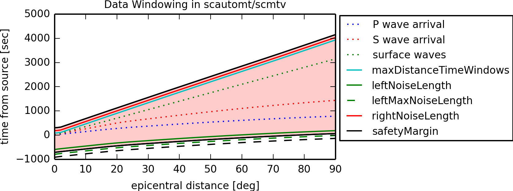
Configuration parameters and time window (red area) with default values used for extracting waveform data and Green’s functions.
Phase-dependent time windowing: The waveforms of seismic phases used for inversion are searched within the initial time window. The start and the end of the phase time windows relative to origin time can be defined per phase individually separately for every profile, e.g.,
automt.profiles.$name.signalBegin.body.Pandautomt.profiles.$name.signalEnd.body.Pfor P waves. If the times are undefined, standard values apply. If the times are defined, they are either read from actual phase picks or from a travel-time table. Read the section Alignment with observed waveforms for the details.For surface waves, LQ and LR, the begin of the time windows initially align with
 and
and  , respectively, where OT
is origin time and d is epicentral distance in degree. Where the resulting
begin time is before the begin time of time windows of S phases, the latter is
used also for surface waves. This may be the case for observations at short
epicentral distances and sources with greater depths.
, respectively, where OT
is origin time and d is epicentral distance in degree. Where the resulting
begin time is before the begin time of time windows of S phases, the latter is
used also for surface waves. This may be the case for observations at short
epicentral distances and sources with greater depths.
The following table shows the standard values relative to origin time for each wave type.
Type |
Begin time |
End time |
|---|---|---|
P |
P-maxShift |
sP+90s+maxShift |
S |
S-maxShift |
S+200s+maxShift |
Rayleigh |
LR-maxShift |
END OF DATA |
Love |
LQ-maxShift |
END OF DATA |
W-phase |
P-30s |
P+15*distance |
Full |
custom(0) |
custom(300) |
The END OF DATA time (EOD) is defined by a configurable function of distance
which is to be added to origin time. EOD is configurable by
automt.data.maxDistanceTimeWindows. The defaults are:
Distance (km) |
EOD (s) |
|---|---|
0 |
80 |
200 |
100 |
2050 |
832.5 |
4050 |
1617 |
6050 |
2392.5 |
8050 |
3164 |
10050 |
3953 |
12050 |
4720 |
14050 |
5506.5 |
16050 |
6234.5 |
18050 |
7011 |
20500 |
8000 |
Centroid depth search
The centroid depth can be determined for a given fixed epicenter by scmtv.
CMT: 3D-centroid search
The 3D-centroid moment tensor (CMT) and its location can be determined
interactively by scmtv and or automatically by
scautomt. The latter requires configuration of
automt.centroid.enabled.
The depth search is defined by automt.depthSearchGrid and
automt.depthFineSearchIncrements.
The Centroid location with the highest fit is selected.
For inspecting the 3D centroid solutions interactively, start the Centroid search in scmtv.
Single inversion quality
An inversion is made for each waveform snippet/item (data of a certain wavetype
on a certain component) on the vertical and radial component. If the best
Fit is below the configured minimum item fit
(automt.profiles.$name.minItemFit), the item (trace, wave
snippet) is removed from further processing. Tangential items are removed along
with radial components of the same wave type.
Solution Fit
The goodness of an inversion is measured by the Fit (goodness of fit, GOF).
Two different methods are available for computing the Fit. The method can be
configured by automt.GOF:
internal (
automt.GOF= internal):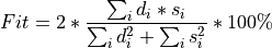
variance reduction (
automt.GOF= varred): The fit function according to Minson and Dreger, 2008.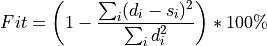
with
 : data sample
 : samples of synthetics (Green’s functions).
Note
Fit is used as a measure of goodness in the Centroid depth search of scmtv.
Solution Quality
In addition to Fit, the Quality parameter as shown
in the depth search widget of scmtv is measured
as the product of Fit and the ratio of the number of used stations  vs. the number of stations available
  for the inversion:
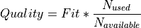
Due to optional optimization during inversion stations with insufficient station fit can be removed and the number of used stations can be removed. When leaving only very few stations after optimization, the Fit may become high while the Quality increases.
Note
Quality of used as a measure of goodness in 3D-Centroid search.
Moment-tensor decomposition
The moment tensor can be decomposed into components representing physical processes:
DC, double-couple: shear sources, e.g. tectonic earthquakes
ISO, isotropic: sources of volume changes, e.g. explosions or implosions
CLVD, compensated linear vector dipole: complicated sources, e.g. ring faulting, rupturing bent faults, collapse of caveties.
DC and CLVD form the deviatoric moment tensor (DEV). The magnitude of the components is typically given as a percentage (%).
For the decomposition different methods are available:
Default: Decomposition by Silver and Jordan [14]. This is the default.
MTDecomp100: Decomposition by Knopoff and Randall [11]. relating all components separately to the total seismic moment of the event.
Default
By default the moment tensor is decomposed into the deviatoric (DEV) and isotropic (ISO) components where DEV is related to the total seismic moment according to Silver & Jordan (1982). The deviatoric part contains the double-couple (DC) and the compensated linear vector dipole (CLVD) such that

and

MTDecomp100
Another type of decomposition relates all components individually to the total seismic moment (Knopoff and Randall [11]):

Activate automt.MTDecomp100 for using this type of decomposition in addition.
In scmtv this decomposition can be optionally selected from the
Options menu.
Note
This method exists currently only for testing. The calculated moment-tensor components are not included in the resulting focal mechanism parameters which are saved.
Scalar moment, M0
The scalar moment, M0, is the tensor norm of the seismic moment tensor.
Magnitudes, Mw
Considering the scalar moment, M0, derived from the moment tensor, the moment magnitude, Mw, is computed as

Magnitudes, Ms(BB)
For each station, the Ms(BB) magnitude is computed from normalized station amplitudes and displayed in the waveform editor.
Quality Control
Before and during inversion of waveforms for moment tensors, measures of waveform and solution quality are taken and applied. Waveforms are evaluated per trace or station.
Clipping detection
A trace is marked as clipped if its maximum raw amplitude exceeds 90% of 223 assuming a 24bit datalogger. Clipped traces are removed from further processing.
Incomplete data
A trace is removed from processing if its data length (according to the signal length function) is less than its lower filter period.
Signal to noise ratio
The signal to noise ratio, SNR, for each wave type with all three components is computed as
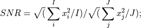
where
x: data sample
i, I: the sample index and number of samples of the signal
j, J: the sample index and number of samples of the noise
If SNR falls below the configured minimum SNR
(automt.profile.$name.minSNR.[type]) all station items of that wave
type are removed from further processing.
Amplitude outliers
For all remaining stations a normalized station amplitude A is measured as the maximum of all available amplitudes on all components of that station. The median is computed over all normalized station amplitudes. Stations are removed from processing where the absolute difference of the normalized amplitude and the median is larger than twice the variance.
Normalized station amplitudes are also used to compute Ms(BB) station magnitudes.