Input Waveform Data
Measured waveform data is provided to the moment tensor modules by configuration of the RecordStream interface through the global recordstream parameter. The RecordStream interface typically considers local or remote waveform archives or servers or miniSEED files.
The data is requested in time windows which
depend on considered phase type and epicentral distance. The data
source is configured through the RecordStream interface.
When fetching the data stations with epicentral distance up to
automt.maximumDistance are considered.
The data processing is described in section Algorithms.
Green’s functions
During inversion of measured seismograms for moment tensors the waveforms are compared with synthetic seismograms, the Green’s functions. Green’s functions are a set of pre-computed displacement waveforms for three fundamental sources representing a deviatoric point source: vertical strike-slip (SS), vertical dip-slip (DS) and a dip-slip with 45° of dip (DD) or an isotropic source (EP). The displacement waveforms take units of cm.
A set of Green’s functions must be made available for nodes at a specific distance and depth as well as a time window. In between nodes, the Green’s functions will be interpolated. The required distance and depth ranges as well as the distance-dependent time windows are configured in scautomt and scmtv.
Each set of Green’s function consists of at least 8 components: ZSS, ZDS, ZDD, RSS, RDS, RDD, TSS and TDS where Z, R and T refer to the vertical, radial and tangential components. For computing the full moment tensor, 2 additional components are required: REP, ZEP. The sample rate of the Green’s functions is used to automatically resample the observed waveform data. It must therefore be high enough to sample the frequency content of observed waveforms in a range which depends magnitude.
SeisComP supports by default two Green’s function formats:
sc3gf1d: SeisComP-native format for Green’s functions for 1D Earth models. This is the recommended and most widely-used format.
Helmberger: An alternative format for 1D media.
Available sets
Along with the mt package gempa provides one set of Green’s functions. Available sets are given in table below. Normally, gemini-prem is delivered. For installation and configuration follow the instructions in the sections Installation and Configuration, respectively.
Name |
Earth model |
sample rate [sps] |
distance range [km] |
depth range [km] |
format |
|---|---|---|---|---|---|
gemimi-prem |
PREM |
1 |
10 - 10,000 |
2 - 700 |
sc3gf1d |
gemini-iasp91 |
IASP91 |
1 |
10 - 10,000 |
2 - 700 |
sc3gf1d |
qseis_ak135f_continental |
ak135 |
1 |
10 - 10,000 |
2 - 700 |
sc3gf1d |
qseis_ak135f_continental |
ak135 |
1 |
10 - 10,000 |
2 - 700 |
sc3gf1d |
gf-qseis-iasp91-16hz |
IASP91 |
16 |
0 - 199 |
0 - 100 |
sc3gf1d |
Custom sets
For monitoring of earthquakes at local and regional scale it may be advantageous to use Green’s function based on locally valid velocity models and higher sample rates. The computation of the Green’s functions must follow notations used in the publication by Minson and Dreger [12]. The Green’s functions can be calculated using any available program for calculating full waveforms in 1D or 3D heterogeneous media. Alternatively, gempa GmbH may be contacted for providing the Green’s functions. Once custom Green’s functions are available they can be added and configured as set out in section Configuration.
sc3gf1d
File Format
This is the recommend format and structure for providing the Green’s functions following the notations in Minson and Dreger [12]. The sc3gf1d format stores the displacement in SAC files.
File and Directory Structure
The general file and directory structure contains
a description file ending on
.descandactual Green’s functions as component files (all other files)
as follows:
[name].desc
[name]/[depth]/[dist]/[depth].[dist].ZSS
[name]/[depth]/[dist]/[depth].[dist].ZDD
[name]/[depth]/[dist]/[depth].[dist].ZDS
[name]/[depth]/[dist]/[depth].[dist].RSS
[name]/[depth]/[dist]/[depth].[dist].RDD
[name]/[depth]/[dist]/[depth].[dist].RDS
[name]/[depth]/[dist]/[depth].[dist].TSS
[name]/[depth]/[dist]/[depth].[dist].TDS
[name]/[depth]/[dist]/[depth].[dist].REP
[name]/[depth]/[dist]/[depth].[dist].ZEP
[name]: name of the set of Green’s functions which is provided. The set is located in the directory defined by
gfaUrland configured byautomt.gfModelin scautomt.
[depth]: depths in units of 100m, format: (%4.4i)
[dist]: epicentral distance in units of kilometers, format: (%5.5i)
Each component file is a SAC record and the unit of the samples is expected to be in units of cm. The suffices indicate the components. Different sets are required for the inversion:
Inversion for deviatoric moment tensors (5 elements, tr(M)=0) requires 8 components:
ZSS, ZDD, ZDS, RSS, RDD, RDS, TSS, TDS
Inversion for full moment tensors (6 elements) requires 10 components:
ZSS, ZDD, ZDS, RSS, RDD, RDS, TSS, TDS, REP, ZEP
The description file name.desc contains a general description of the
archive and an optional definition of the travel-time interface. In particular
the available depths and distances. Units are kilometer.
# depth [from] [to] [step]
depth 10 30 2
depth 30 700 10
# distance [from] [to] [step]
distance 10 10000 10
# travel times
times LOCSAT iasp91_scanloc
In the example above the archive contains depth from 10km to 30 km in steps of 2 km and from 30 km to 700 km in steps of 10 km. Distances are stored from 10 km to 10000 km in steps of 10 km. The line starting with times specifies the travel-time interface and the profile considered for predicting arrival times. Both must exist. The predicted times are shown in the waveform window of scmtv and used for aligning measured waveforms with Green’s functions.
Note
The specification of the travel-time interface by the line starting with times is optional. If missing, libtau with iasp91 is considered.
Timing
Times of the Green’s functions are relative to source time. The source time is 01-JAN-1970 00:00:00. It must be considered for setting the start times in the SAC files when computing Green’s functions with leading samples or when considering reduced times. The start time t of the Green’s functions is then
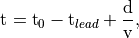
where  : source time,
  : lead time,
 : distance,
  : reduction velocity.
While lead times may be useful to optimize later data processing, time reduction helps to reduce the time length of the computed Green’s functions. Typically, lead times of 200 s and no time reduction are applied to compute Green’s functions at 1 Hz sampling.
Alignment with observed waveforms
Initially, Green’s functions and observed waveforms are aligned in time based
on configured times windows. When time windows are set relative to phase
arrivals, e.g. by automt.profiles.$name.signalBegin.body.P and
automt.profiles.$name.signalEnd.body.P, then measured pick times and
phase arrival times prediced by travel-time interfaces are considered:
For Green’s functions, the arrival times are provided by the travel-time interface.
For measured waveforms the measured pick time is used. If the pick time is unavailable, the time is predicted by the travel-time interface.
The travel-time interface is defined through the description file in the Green’s functions directory. When selecting Green’s functions interactively in scmtv the travel-time interface is reloaded accordingly.
Helmberger
File Format
This format is a simple ASCII format where each depth/distance pair is stored in one file.
File and Directory Structure
The general directory layout looks like this:
name.depths
name.dists
name.vel
name/name[dist]d[depth].disp
The file name.depths contains the information about the available
depths in km as a simple list, e.g.:
0002
0004
0006
0008
0010
0020
0030
0040
0050
The file name.dists contains all available distances in km per depth.
0020
0025
0030
0035
0040
0045
0050
0055
0060
0065
0070
0075
0080
0085
0090
0095
0100
Timing
The optional file name.vel defines the reduction velocity.
The reduction velocity is used to cut the displacement traces (*.disp).
If the file is not given a reduction velocity of 9 km/s is assumed.
The reduction velocity v defines the start time t of the Green’s functions
at distance d with respect to source time.
It is used to compute the time stamp of the
first displacement sample by dividing the distance with the velocity:

The file name.vel just contains one number which is the used reduction velocity
in units of km/s.
File Format Description
Each Green’s function is stored according to the above naming convention in a separate ASCII file. The format is quite simple and contains 8 blocks for each component in the order: TSS, TDS, RSS, RDS, RDD, ZSS, ZDS and ZDD. The file starts with a two line header:
       8
(6e12.5)
The first line contains the number of components stored which must be 8 otherwise the file is not used by scautomt. The second line defines the format for each displacement sample in format ([n]e[w].[d]) where n is the number of samples per line, w the total width of a sample and d the number of digits. The format specifier ‘e’ stored each number with exponent of base 10.
After the initial two lines the block header starts:
0.0000e+00     0.0000e+00      0  0  0.00
1024   1.00000  0.0000e+00
The first line is ignored and from the second line only the first two values are used specifying the number of samples in this block and the sampling time in seconds.
Then a block starts:
-0.00000e+00-4.20540e-10-8.70203e-10-1.12867e-09-1.39191e-09-1.46233e-09
-1.54311e-09-1.43806e-09-1.36765e-09-1.10546e-09-9.15074e-10-5.57482e-10
-3.14872e-10 5.65648e-11 2.74140e-10 6.01314e-10 7.13883e-10 9.43205e-10
...
All subsequent blocks follow continuously (no empty lines).
Configuration
Store the set of Green’s function in some location, preferable the default
directory of gfaUrls and gfaUrl.
Provide the type (format) and the location of the Green’s functions by
configuration of a URL. For the type use sc3gf1d or helmberger depending on
the Green’s functions.
scmtv: Configure
gfaUrlsfor type and location:gfaUrls = [type]://[location] gfaUrls = sc3gf1d:///home/data/greensfunctions
scautomt: Configure
gfaUrlfor type and location andautomt.gfModelfor the model name:gfaUrl = [type]://[location] gfaUrl = sc3gf1d:///home/data/greensfunctions automt.gfModel = gemini-prem