Low-Magnitude Events

While the MT packages generally ships with Green’s functions supporting observation of large (M>5) events inverting waveforms of lower-magnitude events for moment tensors is supported as well by scmtv and scautomt. Since inversion for moment tensors of such events is generally challenging a few requirement must be met:

• High-quality, low-noise waveforms,

• Green’s functions for an appropriate Earth’s model sampled at a rate high enough to represent the frequency content of the inverted waveforms.

• Appropriate travel-time tables for ideally corresponding to the Green’s functions. Define the travel-time tables in the description file of the Green’s functions.

• Create of use an inversion profile specifically configured for smaller events. scmtv ships with two example profiles, FWF3, M3 which are specifically designed for M<3 events. These profiles can be used for reference but eventually tailoring may be required.

  Note

  • In the list of recommended configuration parameters below, full stands for the wavetype and must be adjusted accordingly.

  • The parameters of the standard profile FWF3 are used in the recommendations and the examples below and can be used as starting point and also applied to scautomt:

    automt.profiles.FWF3.name = "Full WF, <M3, GF >2 sps"
    automt.profiles.FWF3.magnitudes = -INF;3.0
    automt.profiles.FWF3.minItemFit = 60
    automt.profiles.FWF3.maxShift = 2
    automt.profiles.FWF3.shiftStep = 1
    automt.profiles.FWF3.minDist = 0
    automt.profiles.FWF3.minSNR.full = 3
    automt.profiles.FWF3.maxShift.full = 1
    automt.profiles.FWF3.wZ.full = 1
    automt.profiles.FWF3.wR.full = 1
    automt.profiles.FWF3.wT.full = 1
    automt.profiles.FWF3.wNormalize.full = true
    automt.profiles.FWF3.periods.full = 1-2
    automt.profiles.FWF3.signalBegin.full = P-1
    automt.profiles.FWF3.signalEnd.full = S+5
    

  Recommendations for inversion profiles:

  • Use full-waveform inversion for time windows covering P and S waves if S-P travel time are well represented by Green’s functions. Otherwise create separate time windows. In order to consider P and S waves equally on 3 components, you may consider P wave time windows in the configuration of full waveforms and S phases by configuring body waves with P and S but a time window only around S phases. The latter is reasonable since inversion of body waves P and S considers vertical and horizontal components separately.

  • Consider small periods (large frequencies) representing the signal’s frequency content. The periods must be supported by the Green’s functions. Configure similar: automt.profiles.$name.periods.full = 1-2.

  • Define precise time windows considering the period range for inversion. Larger periods require larger time windows. Configure similar: automt.profiles.$name.signalBegin.full = P-1 and automt.profiles.$name.signalEnd.full = S+5.

  • Allow only small time shifts of source time and for individual wave snippets. Configure automt.profiles.$name.maxShift and automt.profiles.$name.maxShift.full.

  • Require reasonable Fit of snippets (items). Configure: automt.profiles.$name.minItemFit.

  • Consider high-quality waveforms only. Configure: automt.profiles.$name.minSNR.full.

Interactive inversion

The recommended steps to take for interactive inversion in scmtv are demonstrated with a Mw=2.7 event, observations up to 1.6 degree epicentral distance in central Germany and the inversion profile FWF3:

1. Load the waveforms of an event of interest

2. Unless automatically done, you should now load the set of custom Green’s functions with high sample rates. The data is resampled to the sample rate of the Green’s functions.

   

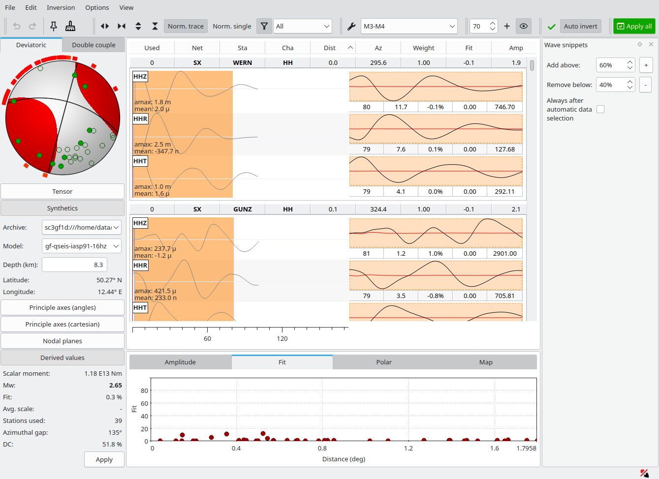
   Initial solution for an ML=3.0 event, Green’s functions for the IASP91 Earth’s model sampled at 16 Hz. Data processing is based on the standard M3-M4 inversion profile.

3. Choose an inversion profile and perform a single inversion. You should test and adjust the profile parameters and eventually store the profile parameters accordingly in the configuration of scmtv

   

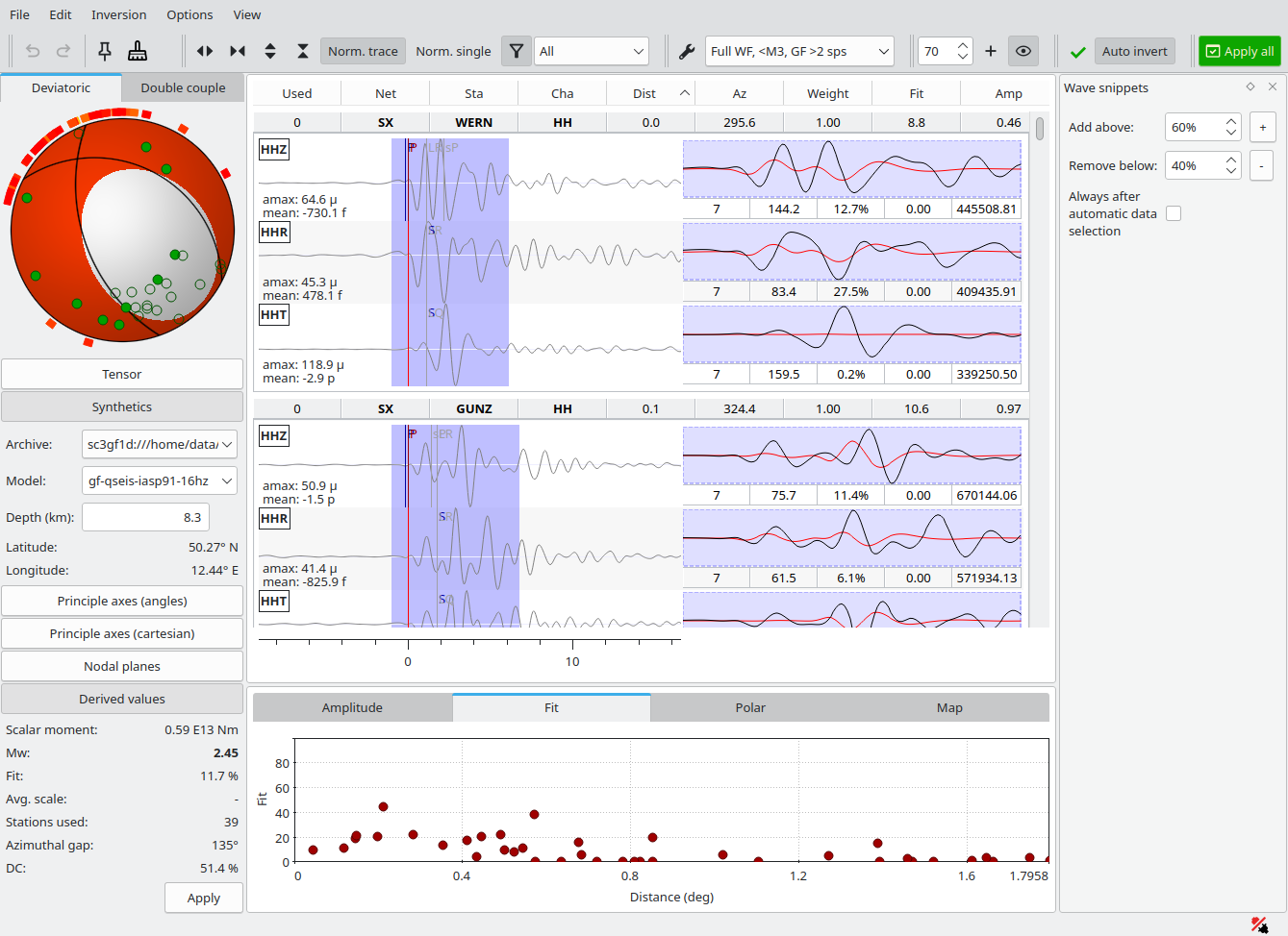
   Initial solution of the same event after loading the standard FWF5 inversion profile. The fit is still poor since waveforms must still be aligned with Green’s functions and noisy data are to be removed.

4. Remove all wave snippets with low Fit, let’s say <40% and trigger a single inversion. If the solution is well-posed, you may add more wave snippets with larger Fit, let’s say >60% and invert again.

   

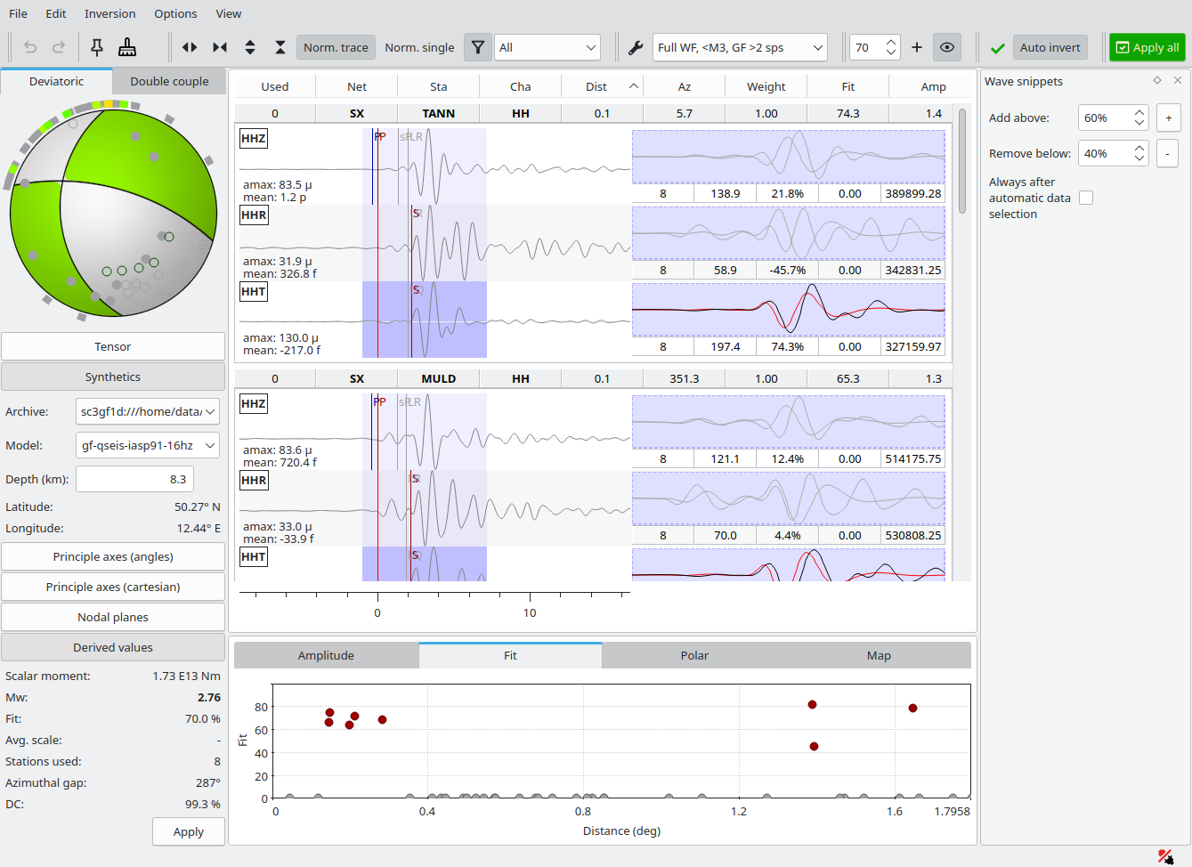
   Solution after removing snippets with Fit <40% and inverting. The overall Fit has improved significantly but the trace alignment is still imperfect.

5. Manually shift the wave snippets to match the Green’s functions and invert again. You may trim the data to discard noise. During shifting and trimming you may activate Norm. Single for a better view on the matched data.

   

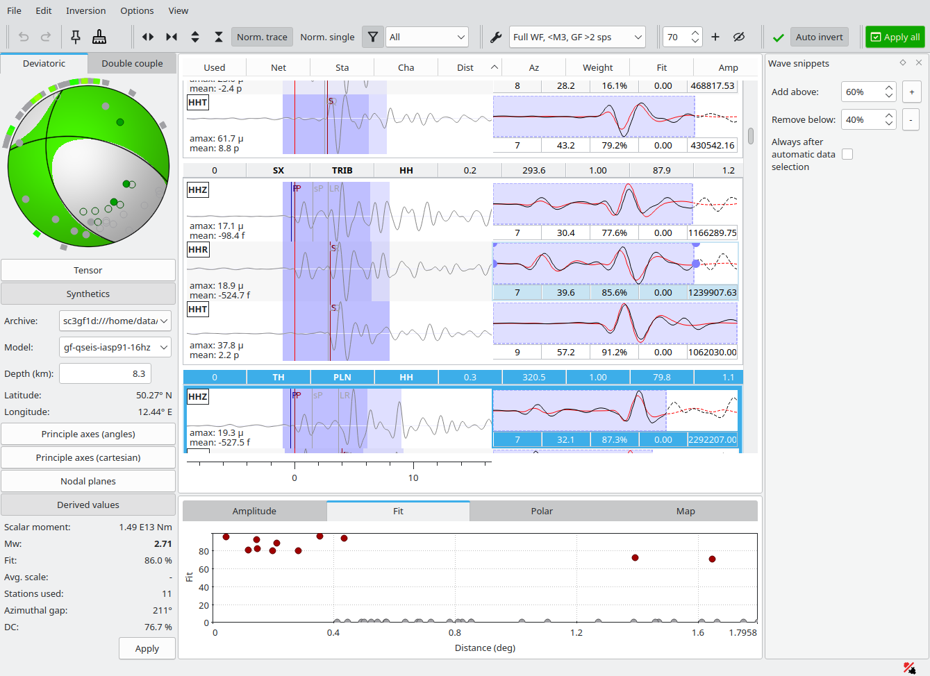
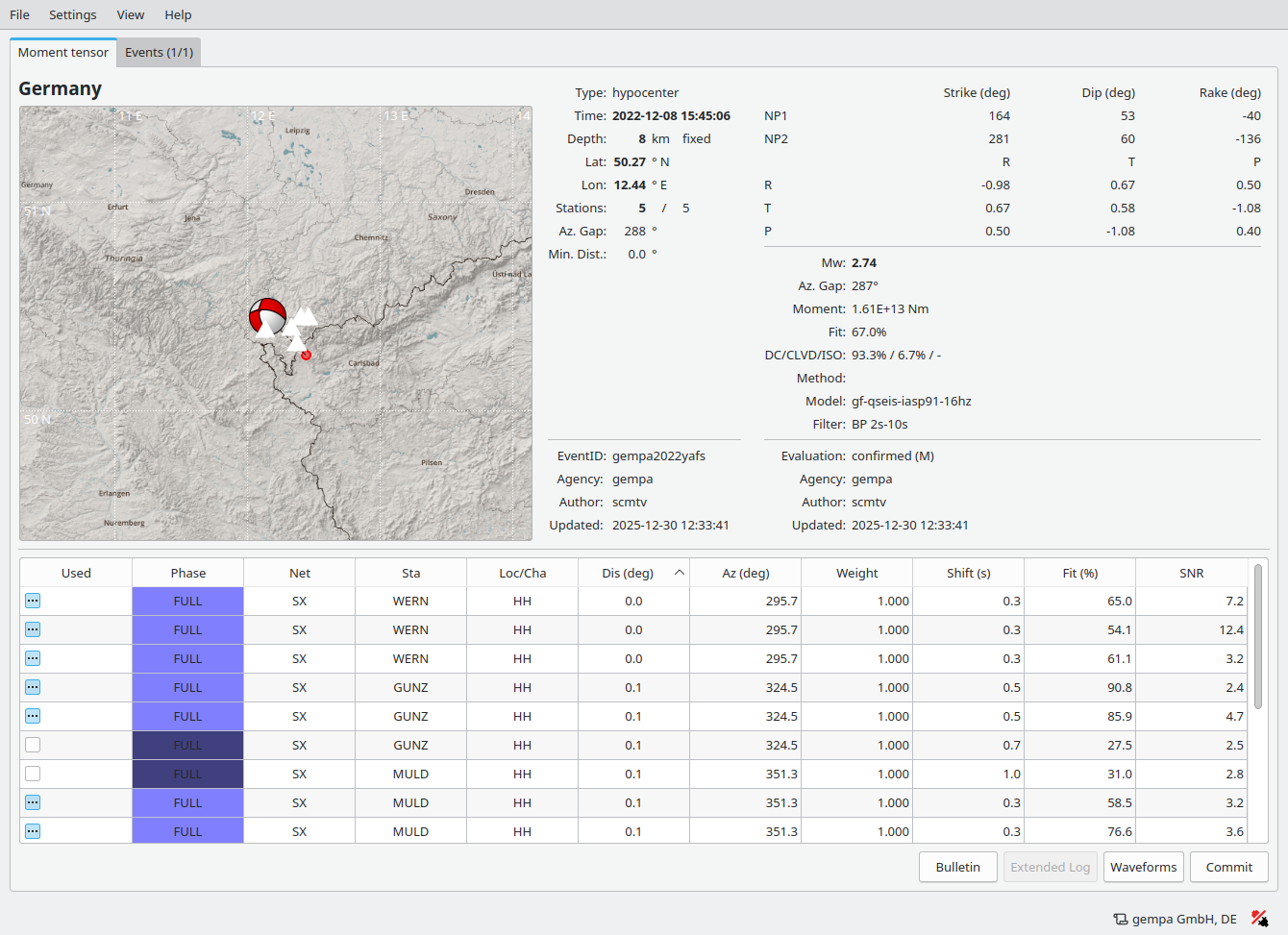
   Final solution after shifting and trimming data. More snippets, previously with low Fit could be re-activated and matched contributing to a stable solution with high Fit and DC (double-couple) percentage. The final Mw is 2.7.

6. When sufficient wave snippets are matched and the solution is stable you may press Apply all and commit the solution.

   

   After applying the solution you may press the Commit button to store the results or generate bulletins and reports.

Automatic inversion

Once the inversion has been tested and verified interactively you may copy the inversion profile parameters to the module configuration of scautomt and run the module without interaction. Before, you may finally test the module in a playback.