Tutorial: a week of Alaska picks

This tutorial builds a reviewed catalogue from one week of automatic picks of the Alaska Earthquake Center (public data of the AK, AV and neighbouring networks): load the picks, nucleate seeds, locate them, remove the false ones with QC rules, merge duplicates, confirm the real ones with the spectra test, review the largest events and send the result. Each step shows the window with numbered markers; the numbers match the list below the figure.

Step 1: Load the picks

Choose the profile and load one week of picks.

1. Profile: choose alaska. A profile holds the settings of the nucleation, the locator, the association and the QC rules for one network, see Processing profiles.

2. Load applies the profile.

3. Set the database window to 2025-03-01 00:00 - 2025-03-08 00:00.

4. Tick picks only. The catalogue is built from the picks, so no origins are loaded. aggregate stays ticked: it merges picks of the same onset made by several pickers.

5. DB loads the window. A progress dialog shows the loading and the building of the tables; a week of picks takes a few seconds. Afterwards the number of picks appears at the top right of the Picks panel.

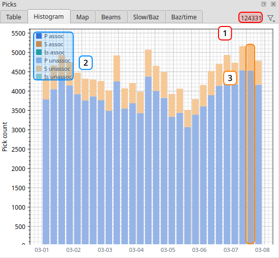
The loaded week in the Histogram tab of the Picks panel.

1. 124 331 picks are loaded.

2. The colours separate associated picks (dark) from unassociated ones (light), per phase family P, S and Is. Without origins every pick is unassociated.

3. Each bar counts the picks of six hours; there are about 3 500 to 5 000. Clicking a bar shows only its picks, see Pick filters.

Step 2: Nucleate seeds with DBSCAN

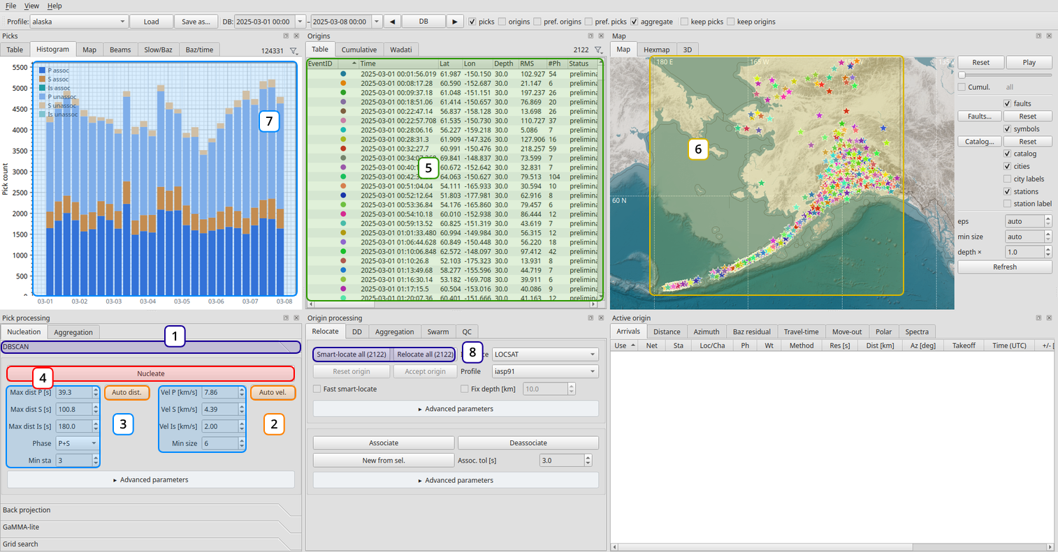
DBSCAN turns the week of picks into 2122 seed origins.

1. In the Pick processing panel open DBSCAN. It clusters picks that are close in time and whose stations are close to each other, see Nucleation.

2. Auto dist. and Auto vel. derive the parameters from well-located origins selected in the origin table. The alaska profile already holds values found this way, so nothing needs to be selected here.

3. Check the parameters: Max dist P / S (39.3 / 100.8 s) is the largest time distance between neighbouring picks, the velocities (7.86 / 4.39 km/s) turn station distances into time. Phase P+S clusters both phases, Min size 6 and Min sta 3 are the smallest cluster that becomes a seed.

4. Press Nucleate.

5. The seeds appear in the origin table: 2122 preliminary origins without an event. They are not located yet: the position is the centre of the cluster, the depth the default of 30 km, and the RMS is large.

6. The map shows the seeds along the Aleutian arc and in southern and interior Alaska.

7. In the histogram most picks are now associated (dark). The light rest belongs to no seed: noise picks and events too small to cluster.

8. The location buttons now count the seeds: Smart-locate all (2122) is the next step.

Step 3: Locate the seeds

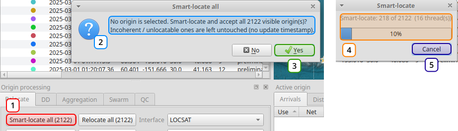
Smart-locate all: confirmation and progress.

1. In the Origin processing panel, tab Relocate, press Smart-locate all (2122). With no origin selected it works on all visible origins. Smart-locate relocates each seed, removes outlier arrivals and tries the alternative phase of doubtful picks, see Refining origins.

2. The confirmation says what will happen: every seed is located and the result accepted. Seeds that cannot be located, or whose picks do not fit one source, stay as they are and are not marked as updated.

3. Press Yes.

4. The progress dialog counts the located seeds; the origins are processed in parallel, here with 16 threads. A week of seeds takes a few minutes.

5. Cancel stops after the origins in progress; the ones done so far keep their new location.

Step 4: Look at the result

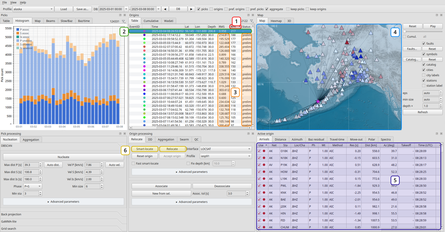
After smart-locate: the origins sorted by phase count, the largest one selected.

1. Click the #Ph header twice to sort by phase count, largest first. The best-constrained origins come to the top; the small ones, where most of the quality control happens later, go to the bottom.

2. Click the top row. It is now the active origin: 217 phases, RMS 0.96 s and a depth of 207 km. The preliminary status is gone: the origin was located and accepted.

3. Some of the large seeds are still preliminary, with a depth of 30 km and an RMS of 100 s and more. Smart-locate left them untouched because their picks do not fit one source. Typical reasons are two events close in time that DBSCAN put into one cluster, or a distant event whose arrivals cross the whole network. These seeds are handled in the next steps.

4. The map shows the active origin (star), the rays to its stations and the stations coloured by their residual.

5. The Arrivals tab lists its picks with phase, weight, residual, distance and azimuth.

6. With an origin selected, the location buttons work on the selection only: Smart-locate and Relocate no longer show a count.

Step 5: Remove the bad outliers with QC

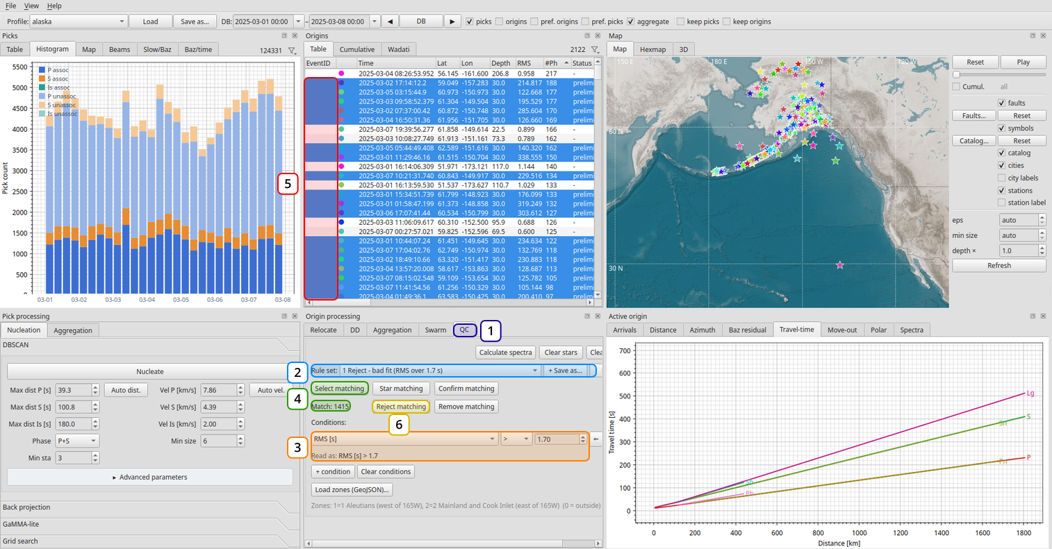
The first reject rule selects the origins with an RMS over 1.7 s.

1. Open the QC tab in the Origin processing panel, see Quality control.

2. Rule set lists the rules of the alaska profile. The reject rules were derived from the confirmed origins of the network, so they hit almost no real event. Start with 1 Reject - bad fit (RMS over 1.7 s).

3. The conditions of the rule, here RMS [s] > 1.70. Read as repeats them as a sentence.

4. Select matching selects the origins that match the rule. Match shows how many.

5. The matching origins are selected in the origin table. Check a few of them before rejecting: click one and look at its travel-time plot.

6. Reject matching sets them to rejected. Repeat with the rule sets 2 and 3.

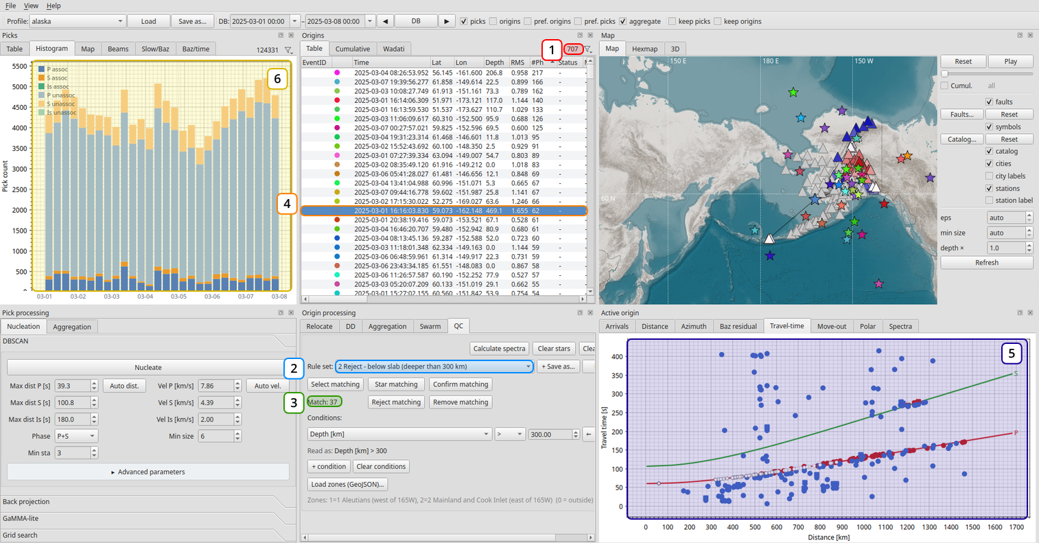
After the first rule: 707 origins left; the second rule finds 37 origins below the slab.

1. Rejected origins are hidden: the origin table now counts 707.

2. The next rule set, 2 Reject - below slab (deeper than 300 km). The Alaska slab has no earthquakes below about 300 km, so deeper solutions are artefacts.

3. Select matching finds 37 origins.

4. Click one of them, here a 469 km deep solution with 62 phases and an RMS of 1.66 s.

5. Its travel-time plot shows why it is wrong: the used P arrivals start at about 400 km distance and there is no S. Without near stations depth and origin time trade off, and the locator moves the source down. Press Reject matching.

6. The histogram shows the price of the first rule: the picks of the rejected seeds are unassociated (light) again. They are not lost, a second nucleation round can use them.

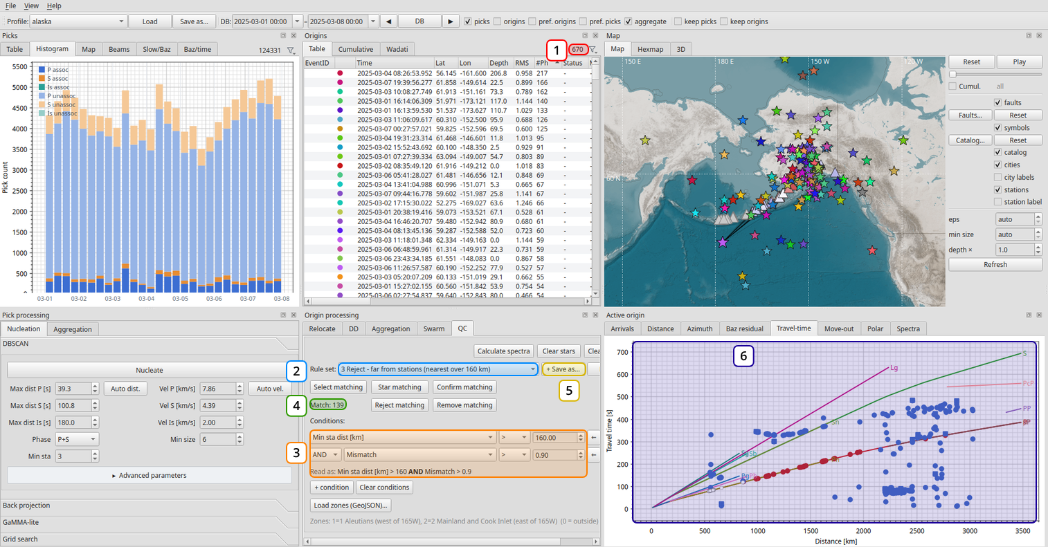
Rule 3 with an extra condition: far from the stations and not seen by the stations nearby.

1. After rule 2, 670 origins are left.

2. Rule set 3 Reject - far from stations (nearest over 160 km).

3. Alone, the distance condition would also hit real earthquakes: along the Aleutian arc and offshore the nearest station is often more than 160 km away. The rule therefore has a second condition, AND Mismatch > 0.9; the alaska profile already contains it. The mismatch is the weighted fraction of the nearby available stations that the origin does not use (0 = all used, 1 = none). A real event far from the network is still seen by the stations closest to it; a false solution far away is not.

4. Select matching now finds 139 origins. Check a few and press Reject matching.

5. For your own rules, + condition adds a condition and + Save as… stores the changed rule in the profile, so it is available next time.

6. The travel-time plot of an offshore origin: the used P arrivals (red) follow the P curve from about 550 km on.

The goal of this step is not a final catalogue, but a smaller set without the obvious false origins: the spectra of the next step load waveforms for every origin, so each origin removed here saves waiting time. Around 500 origins are a good size; in this week the first three rules already bring the 2122 seeds down to 531, so the tutorial continues with them. The rule sets 4 to 8 of the profile work the same way and can be applied in addition; they are not used here.

Step 6: Merge duplicate origins

DBSCAN can produce two seeds for one earthquake, for example when a cluster is split at a gap in the picks. After smart-locate both end up at nearly the same place and time, often with picks in common: the event is in the list twice. Merging them before the spectra saves another waveform request and keeps the catalogue clean.

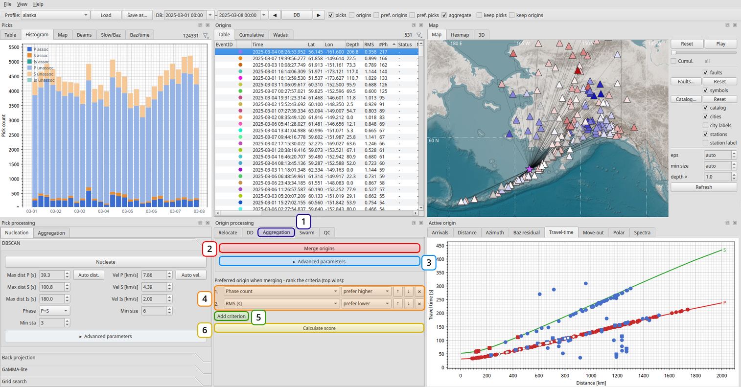
Merging duplicate origins.

1. Open the Aggregation tab in the Origin processing panel.

2. Merge origins combines origins that describe the same event: their hypocentres and origin times are close, or they share enough picks, see Refining origins.

3. Advanced parameters holds the limits: merge distance and time, minimum shared picks and the pick match tolerance.

4. The ranking decides which origin of a group is kept. The criteria are compared from top to bottom: here the origin with more phases wins, and with the same phase count the one with the lower RMS.

5. Add criterion adds another one, for example Author or Method.

6. Calculate score fills the Score column with the origin score plugin, which can then be used as a criterion as well.

In this week merging removes only 6 origins (531 to 525): DBSCAN and smart-locate rarely produce the same event twice. The step is cheap, so it is worth doing anyway before the waveforms are loaded.

Step 7: Calculate the spectra

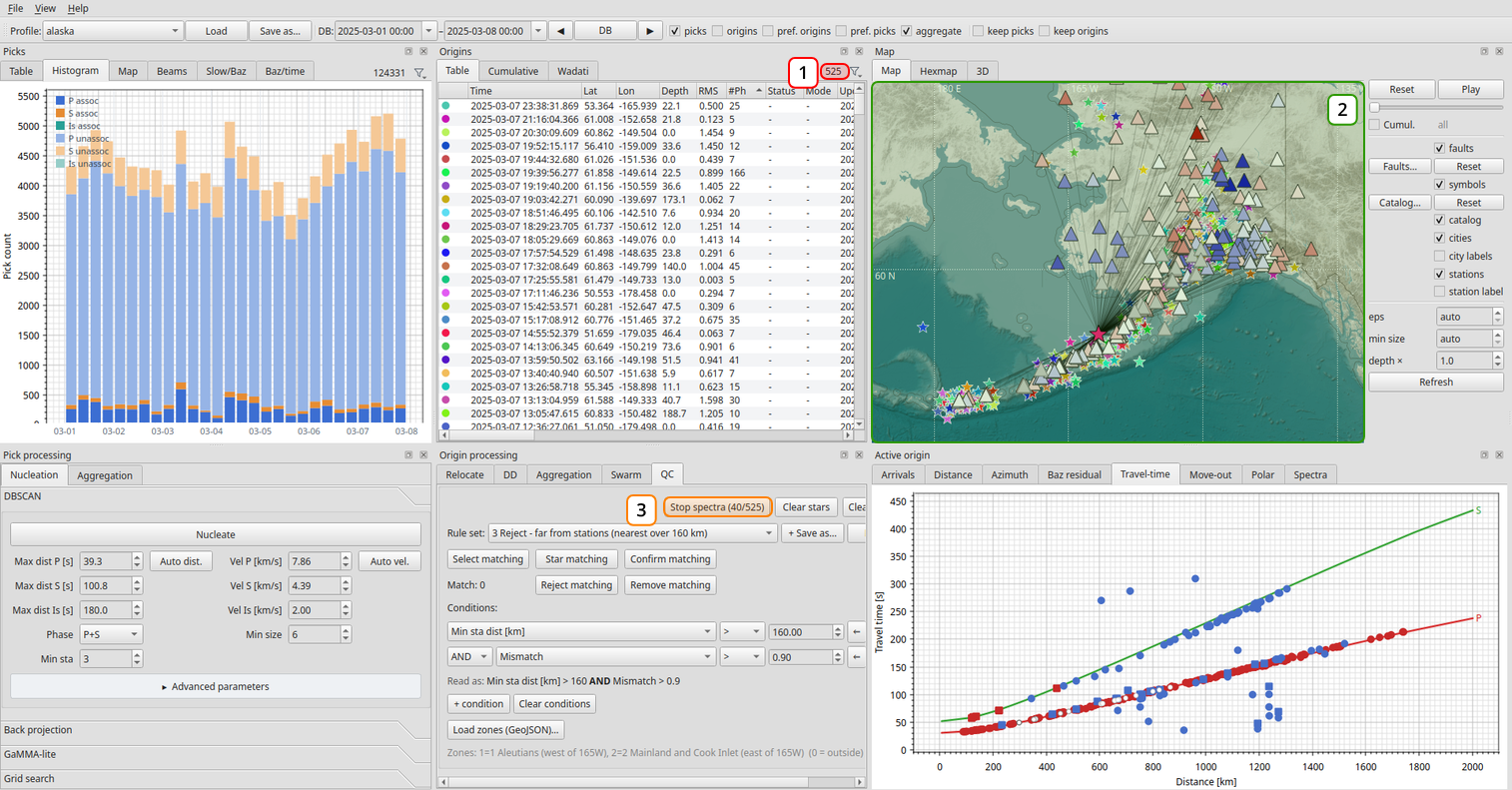
525 origins are left after QC and merging; the spectra are being calculated.

1. The origin table counts 525 origins.

2. The map shows what is left: the Aleutian arc, the Alaska Peninsula, Cook Inlet and interior Alaska, and only a few isolated origins.

3. Press Calculate spectra in the QC tab. Catalyst loads the waveforms of the stations within the profile’s spectra distance (200 km for Alaska) and compares the signal after the origin time with the noise before it, see Spectra and Spectra. While it runs the button becomes Stop spectra with the progress (40 of 525). For the 525 origins of this week it takes 2 to 3 minutes, depending on the connection to the waveform server.

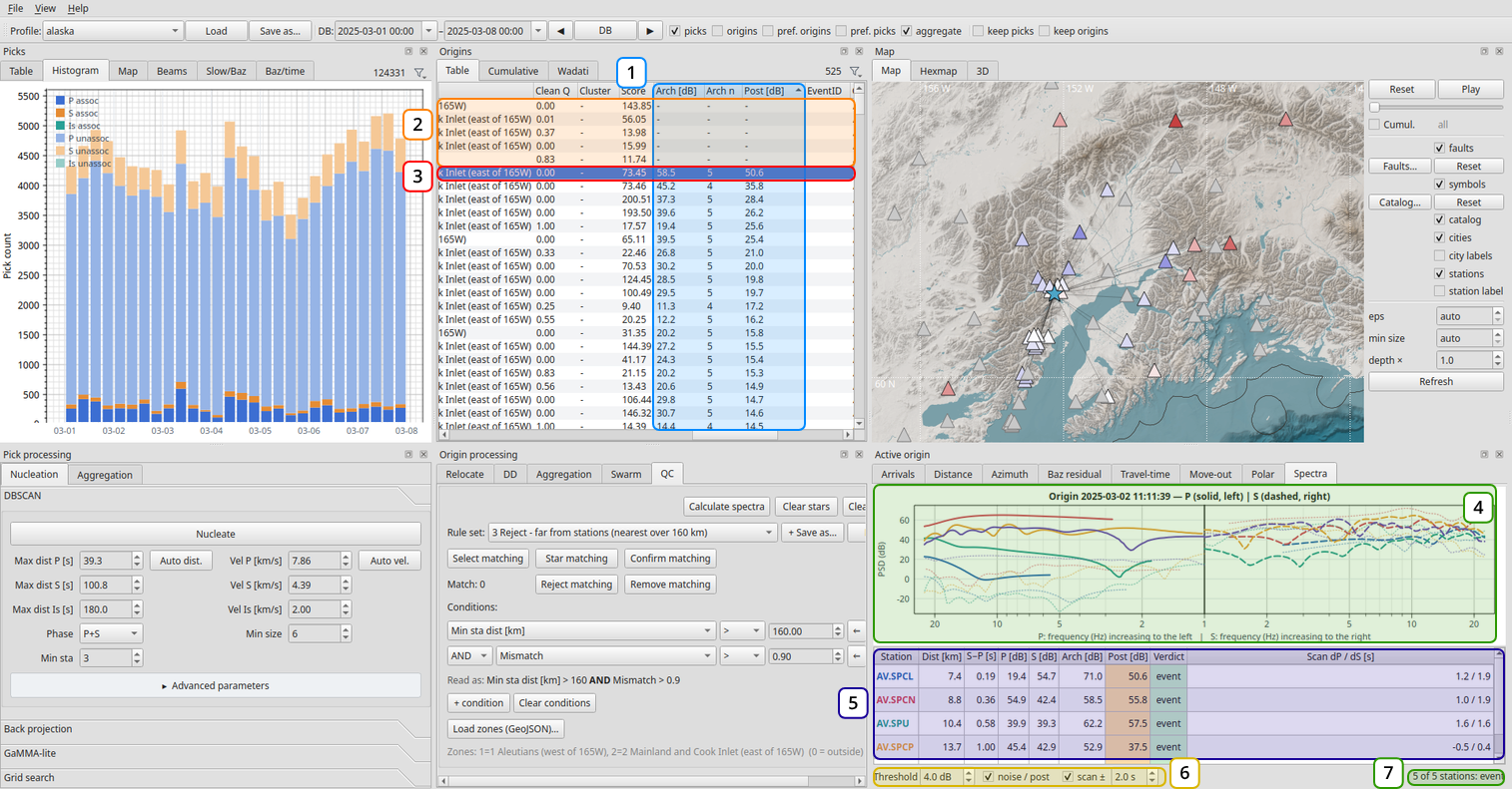
The spectra columns in the origin table and the Spectra tab of a clear event.

1. When the run is done, the origin table has three new values per origin: Arch [dB], the height of the spectra above the noise, Arch n, the number of stations showing an event, and Post [dB], the level of the window after S. Here the table is sorted by Post, highest first.

2. A dash means no value: no station within the spectra distance, or no waveforms. A spectra rule does not match these origins, so they are neither rejected nor confirmed by it.

3. The selected origin: Arch 58.5 dB on 5 stations, a clear event. Its Post of 50.6 dB is high as well: the stations are those of Mount Spurr volcano (AV.SP*), and another small earthquake follows within the window.

4. The Spectra tab of the Active origin panel: for each station the P window (solid, left) and the S window (dashed, right) rise far above the noise (dotted) and form an arch over the middle line.

5. The station table: distance, S−P time, the height of P and S above the noise, the arch, the post level and the verdict per station.

6. Threshold (4 dB in the alaska profile) decides when a station counts as event; scan ± shifts the windows by up to 2 s to absorb small location errors.

7. The summary: 5 of 5 stations show an event.

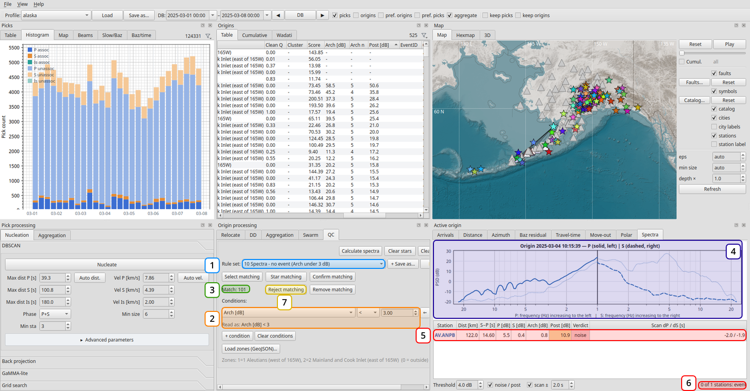
The spectra rule no event and one of its 101 matches.

1. Select the rule set 10 Spectra - no event (Arch under 3 dB).

2. Its condition is Arch [dB] < 3: no station lifts the spectra 3 dB above the noise.

3. Select matching finds 101 of the 525 origins.

4. One of them: the P window (solid) barely rises above the noise (dotted), and in the S window the noise is even higher than the signal. There is no arch.

5. Only one station lies within 200 km, AV.ANPB at 122 km, with an arch of 0.8 dB and the verdict noise.

6. The summary: 0 of 1 stations show an event.

7. Reject matching rejects them. Look at a few first: with a single distant station, as here, a small real event can stay below the threshold too. Such origins are better checked by hand than rejected blindly.

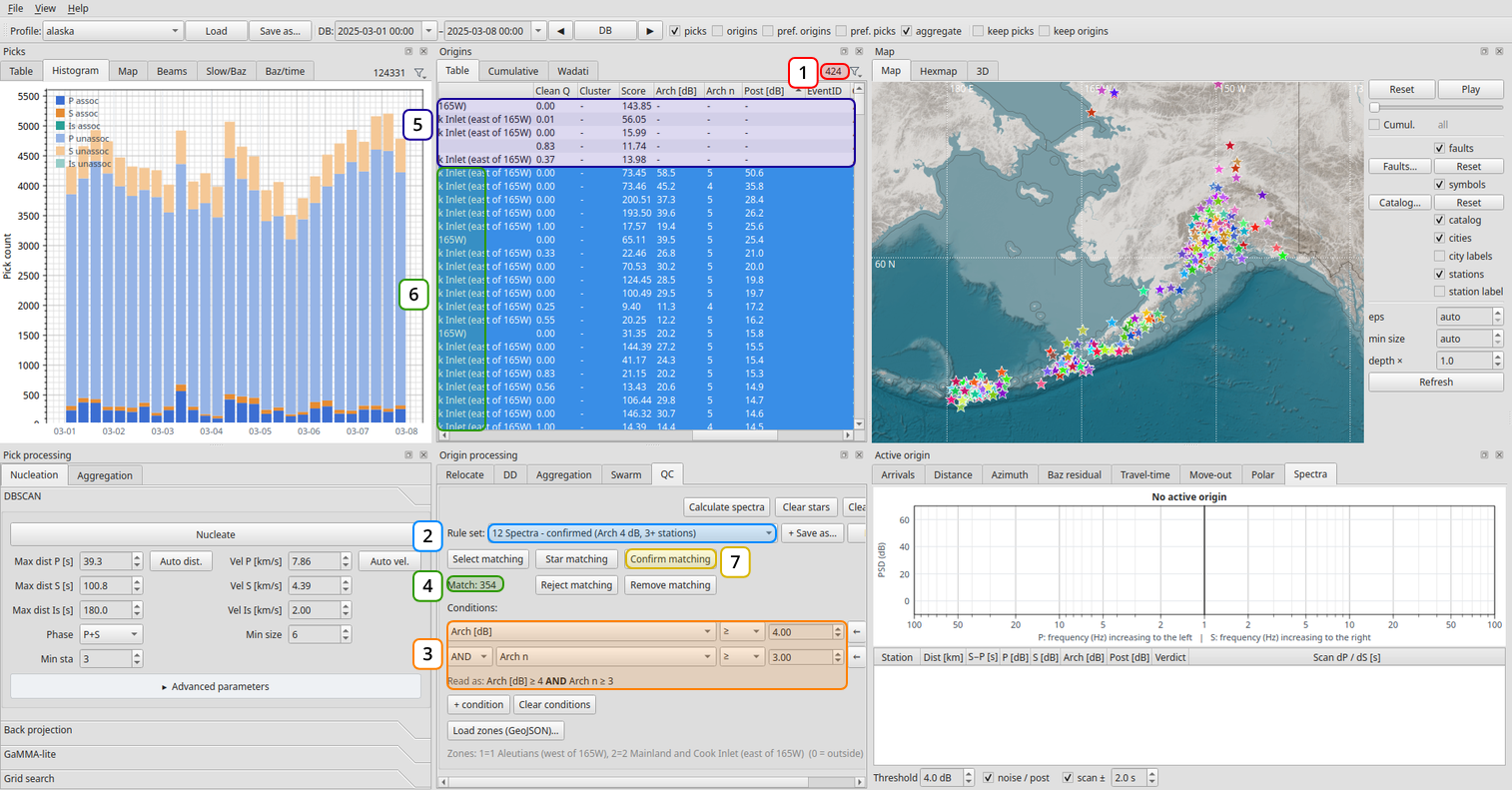
The spectra rule confirmed selects 354 of the remaining 424 origins.

1. After rejecting the 101 no event origins, 424 are left.

2. Select the rule set 12 Spectra - confirmed (Arch 4 dB, 3+ stations).

3. Two conditions: Arch [dB] ≥ 4 AND Arch n ≥ 3, a clear arch on at least three stations.

4. Select matching finds 354 origins.

5. The origins without spectra values (dash) do not match and stay unselected.

6. The matching origins are selected in the table and on the map.

7. Confirm matching sets them to confirmed.

The 70 origins that are neither rejected nor confirmed are the ones worth an analyst’s time: no spectra values, an arch between 3 and 4 dB, or fewer than three stations with an event. Filter on them and check them one by one with the Travel-time, Move-out and Spectra tabs.

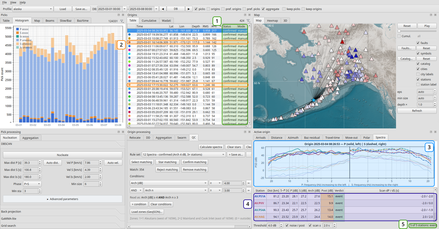
After confirming: the table sorted by phase count again.

1. Status shows confirmed and Mode manual for the confirmed origins.

2. Two well-recorded origins in the Aleutians (142 and 66 phases) are not confirmed: no station lies within the 200 km of the spectra test, so they have no spectra values. They belong to the origins to review.

3. The Spectra tab of the largest origin, 207 km deep below the Alaska Peninsula: a clear arch on all stations.

4. The S−P time of about 23 s at only 80 to 95 km epicentral distance fits the depth: the waves travel more than 200 km to the stations.

5. 5 of 5 stations show an event.

Step 8: Review the large origins

Confirmed or not, the origins with the most phases deserve a look: they are the best-recorded events of the week, and smart-locate may have left picks out that belong to them. Sort by #Ph again and go through them from the top.

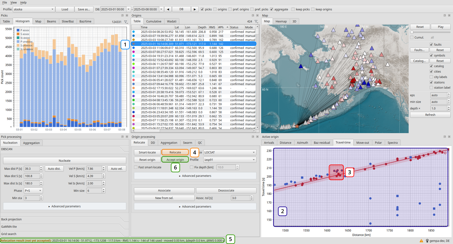
Adding picks that lie just outside the tolerance band.

1. Select the origin, here the Aleutian event of 2025-03-01 16:14 with 142 phases.

2. Zoom into the Travel-time plot, here to 1500 to 1900 km. The used picks (red) follow the P curve inside its tolerance band (shaded). Blue picks are not associated with the origin.

3. Picks just next to the band at the right time are very likely P of this event, missed because of a small travel-time error at that distance. Hold Shift and draw a box around them: they are added to the origin and the arrivals already in use stay. A box without Shift keeps only the picks inside it. A double-click on a single pick adds it as well, see Refining origins.

4. Press Relocate.

5. The status bar shows the result before it is accepted: 144 of 146 arrivals used, the location moved by 0.00 km and the RMS did not change. The added picks fit.

6. Accept origin keeps the result; Reset origin discards it.

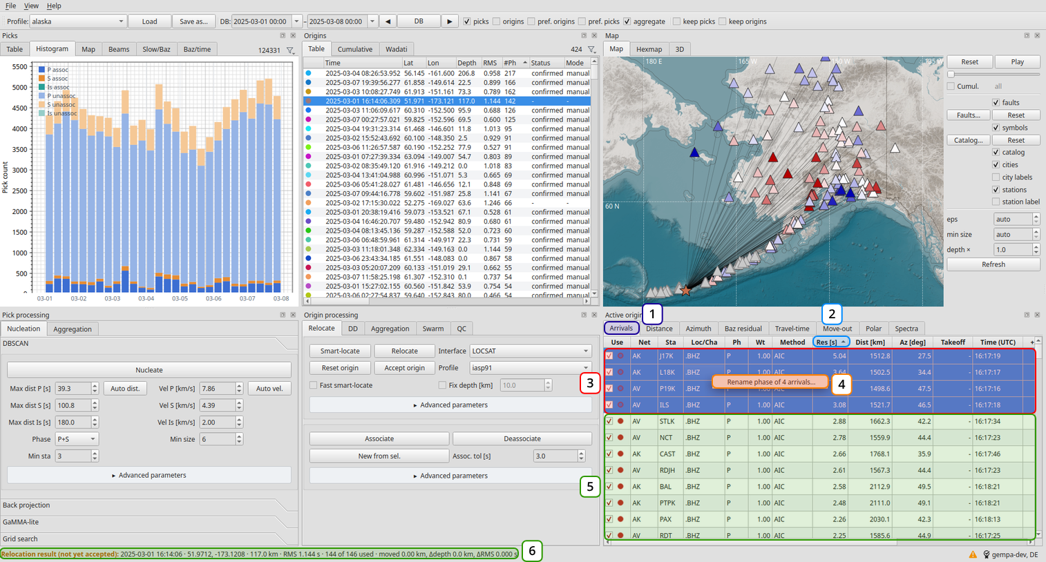
The added picks in the arrival table, sorted by residual.

1. Open the Arrivals tab of the Active origin panel.

2. Click the Res [s] header to sort by residual, largest first.

3. The added picks come to the top: J17K, L18K, P19K and ILS, with residuals of 3.1 to 5.0 s at about 1500 km, just above the association tolerance of 3 s. Their marker (blue inside, red ring) shows a pending add: they are part of the origin from the next relocation on.

4. If an added pick is not a P, select the rows and choose Rename phase from the context menu, see Active origin panel.

5. The arrivals already in use follow with residuals below 3 s.

6. After Relocate the status bar reports 144 of 146 arrivals used and no change of the location: the added picks fit the solution. Press Accept origin.

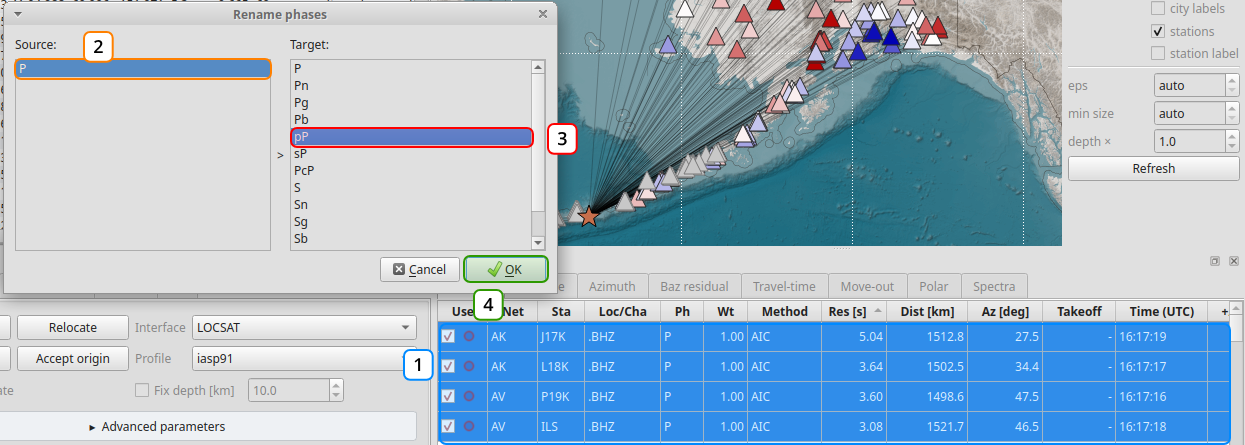
Renaming the phase of the four added picks.

1. Select the arrivals to rename, right-click and choose Rename phase.

2. Source lists the phases of the selected arrivals, here P.

3. Choose the Target phase, for example pP.

4. OK renames them. The locator takes the new phase as given at the next relocation.

Check a rename with the next Relocate: the residuals of the renamed picks must become small. A later phase has its own delay after P; for pP it grows with the depth of the source, about 13 to 15 s for 117 km at 1500 km. A pick 3 to 5 s after P at this depth therefore gets a large residual as pP, while it fits as P. Reset origin undoes the relocation if the rename does not fit.

Step 9: Send the result

Only the confirmed origins go out. Filter the table on them, select them and send them to the messaging system.

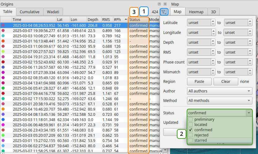
Filtering the origin table on confirmed origins.

1. The filter button in the header of the origin table opens the filters.

2. Under Status tick only confirmed.

3. The table then lists only origins whose Status is confirmed; the count next to the filter button shows how many.

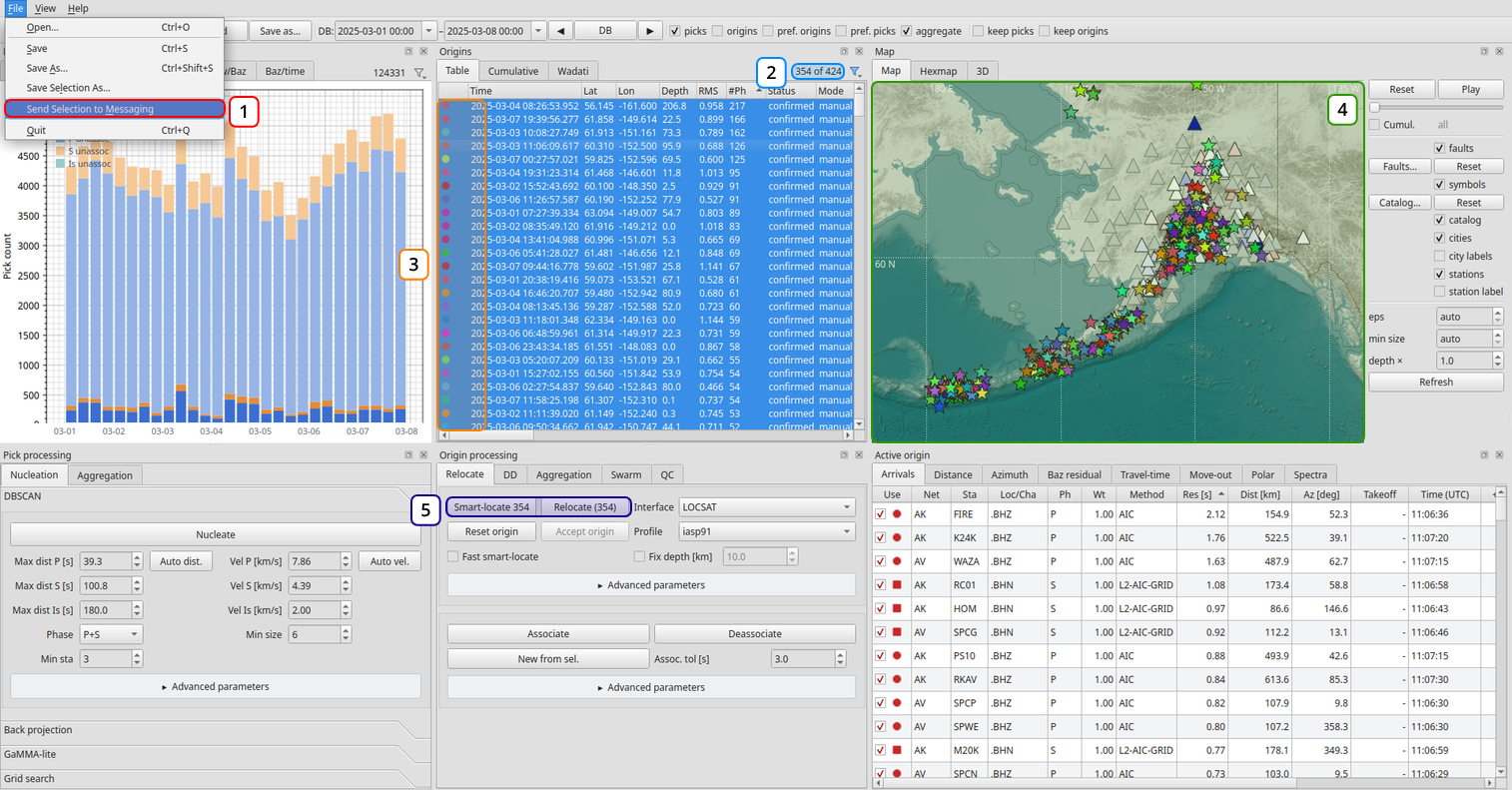
The 354 confirmed origins of the week, ready to be sent.

1. Press Ctrl+A in the origin table and choose File → Send Selection to Messaging. Catalyst sends the selected origins that are new or were changed, with their arrivals and magnitudes, see Send or save the results.

2. The filter shows 354 of 424 origins.

3. All of them are selected.

4. The map shows the confirmed events of the week: the Aleutian arc, the Alaska Peninsula, Cook Inlet and interior Alaska.

5. The buttons count the selection: Smart-locate 354, Relocate (354).

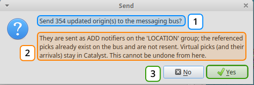
The confirmation before the origins are sent.

1. Catalyst asks before sending and names the number of origins.

2. The origins go out as new objects to the LOCATION group, with their arrivals; the picks they refer to are already in the system and are not sent again.

3. Yes sends them. A progress dialog follows the three stages (collecting, preparing, sending). The sent origins then appear in scolv and the other SeisComP applications.

What you did

In nine steps a week of picks became a reviewed catalogue:

Step	Origins
DBSCAN seeds	2122
After the QC rules 1 to 3	531
After merging duplicates	525
After rejecting no event by spectra	424
Confirmed by spectra	354
Left for review	70

Where to go from here:

• A second round on the remaining picks. The histogram still shows many unassociated picks: noise, small events, and the picks of the rejected seeds. Untick Show associated in the pick filters, so that only these picks are listed, and run another nucleator over them, for example GaMMA-lite, which separates events that overlap in time - the case DBSCAN merged into one seed in step 4. Then repeat steps 3 to 7 on the new seeds: smart-locate, QC, merging, spectra and confirmation. See GaMMA-lite.

• The next week. The arrow buttons next to the database window move it by one week and load it; the profile stays the same, see Toolbar.

• The origins left for review. Filter on the status located and go through them with the Travel-time, Move-out and Spectra tabs.

• Your own rules. Change a QC rule set, test it with Select matching and store it with + Save as…, see Quality control.

• Your own profile. Save as… in the toolbar stores all parameters used in this tutorial, see Processing profiles.