npeval
npeval calculates and reports network performance parameters related to the ability to locate earthquakes.
Description
npeval evaluates and reports important network performance parameters based on network geometry and real-time waveform quality control (QC) parameters. It generates reports of station status and waveform QC parameters which can be reported to external applications, e.g. to GDS [1] for dissemination.
Important features are:
Computes a range of relevant performance parameters describing seismic monitoring networks by different methods.
Station status and QC parameters can be reported, processed and sent to stakeholders.
Considers only stations which are used for the actual event detection based on configurable bindings or stations defined in CSV tables.
Dynamically considers enabled or disabled stations and excludes stations given in a file.
Dynamically considers changes in the station quality control (QC) parameters.
Computation is triggered by significant changes in station status.
Writes computed parameters to Surfer grid files, BNA polygons which can be evaluated on SeisComP maps, PNG images or CSV files.
Configurable are among others:
detection module from a specific processing pipeline or explicit station lists,
minimum number of stations and maximum allowed azimuthal gap for locating earthquakes,
region, grid interval and depths for considering earthquakes,
delay added to the stations considering data transfer and processing,
travel-time table and interface,
random station removal simulating stations not having picks (command-line option),
intervals and colors of contour lines and fill properties,
directory for output,
minimum update interval,
format of generated files: GRD, BNA, PNG, CSV,
output processing script.
Methods
npeval provides multiple methods for computing performance parameters that characterize the seismic monitoring networks in a configurable region:
Minimum time: The minimum time which is required for locating events.
Minimum magnitude: The minimum magnitude of events that can be located.
Number of stations: The number of stations available for detecting events within a configured distance around the events.
S-P travel times: The difference of travel times between P and S phases observed at a point of interest.
Station reports allow archiving, processing or sending relevant network information.
related to the network geometry and the data quality. The methods are applied to the same region simultaneously.
Upon computation of the parameters the output parameters can be stored as surfer GRD, PNG image, BNA or CSV files. For visualizing the grid files dynamically on maps, the plugin mapmultigrid [6] has been developed.
Minimum location time
Computing the minimum times to locate events by a network can be deactivated or
activated by times.compute.
The required configuration is:
Define the minimum number of stations (
stations.stationCount) and the maximum gap (stations.maxGap) as quality measures.Set the parameters for computing the travel times.
times.dataDelay: The time added to the computed travel times considering the data delay measured by scqc [11]. To read the delay from the SeisComP database and to receive dynamic updatestimes.dataDelay = -1.0
Otherwise a static delay is considered.
times.processingDelayData processing time to be added to computed travel times accounting for delays due to the data processing by SeisComP modules, e.g. the detector or the locator. The amount considers the default time window for AIC for phase picking and the default time window for calculating amplitudes for the mB magnitude used by scautopick as well as the processing required by scautoloc [8] or scanloc [7].times.processingDelaymust be therefore be changed when adjusting those window lengths or module configurations.times.file: The base name of the output files.
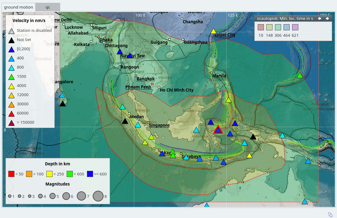
Figure 1: Minimum expected times for locating events in SE-Asia by the GE network.
Minimum magnitude
Computing the minimum magnitude of events expected to be located by a network
can be deactivated or activated by minimumMagnitude.compute.
Different methods for computing minimum are available.
The required configuration is:
stations.stationCount: Define the minimum number of stations.minimumMagnitude.compute: Activate to enable the computation.minimumMagnitude.file: The base name of the output files.minimumMagnitude.type: The Types considered for computations. Currently, supported types are:MDD (magnitude-detection-distance)
LF (low-frequency approximation of the source spectrum, experimental)
GMPE (Ground Motion Prediction Equation, experimental).
Types:
Warning
The types LF and GMPE are currently experimental and may produce results with large uncertainties.
MDD - magnitude-detection distance Considered when
minimumMagnitude.type= MDD. The method assumes that for a given magnitude, P and S phases can be detected up to some hypocentral distance. The magnitude-distance relation is given by (Valtonen et al. [23]):
where:
M: magnitude
D: hypocentral distance enclosing a minimum of stations. The number is configured by
stations.stationCount,
The parameters may be determined from optimization [23] based on reference events for the area of interest. The default values originate from Valtonen et al. [23] for a site in Finnland. Examples from previous optimizations are:
region
a
b
c
Finland [23]
0.001514
0.9327
-1.306
Chile [a]
0.001272
0.887049
-0.065408
Germany/Vogtland [a]
0.001639
1.297967
-1.28476
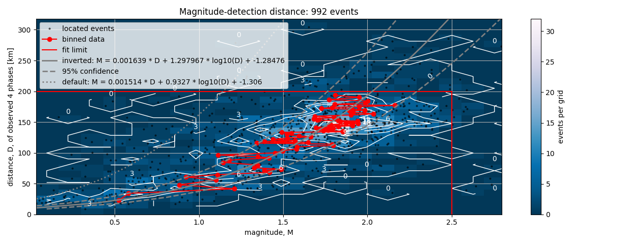
Figure 2: Parameter optimization based on events in Germany/Vogtland [a].
LF - low-frequency-approximation: Considered when
minimumMagnitude.type= LF. Results are specifically sensitive to:Earth’s properties at the hypocentre and along the P wave as well as the stress drop due to the event. The method is adapted from the publication by Tramelli et al. (2015) [20].
travel times computation to account for anelastic attenuation.
magnitude range defined by
minimumMagnitude.magMinandminimumMagnitude.magMaxand the intervals byminimumMagnitude.magStep.
- *.
minimumMagnitude.minSnrdefining the minimum signal-to-noise ratio (SNR) which the data must exceed for a station to be considered. The SNR is calculated by dividing the amplitude predicted by npeval by the data RMS measured by scqc [11].
GMPE - GoundMotionPredictionEquation: Considered when
minimumMagnitude.type= GMPE. The method uses an internally defined GMPE based on the publication by Cauzzi et al. [16]. Choosing GMPE is currently experimental only experimental and not recommended for routine processing.
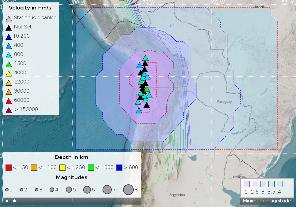
Figure 3: Minimum expected magnitude of events for which a solution can be expected in Chile by the CX network.
Note
Applying the type LF to the minimum magnitude method requires waveform RMS
to be available from real-time station QC messages or from a station input
file (see command line option --file).
Number of stations
The number of station are counted that are available within some hypocentral
distance around a grid point is counted. The distance is configured by
nStations.maximumDistance. Alternatively, the distance is estimated
from a magnitude if configured in nStations.magnitude. Activate
nStations.compute for applying this method.
S-P travel times
The travel-time differences between first arriving P and S phases are computed at points of interest (POIs) assuming events defined on the configured grid. In an earthquake early warning (EEW) system, the method may be used to estimate the remaining alert time at a POI in case a P phase was detected.
Configuration;
Adjust the parameters controlling the travel-times computations in the travelTimes parameter groups,
Add profiles of points of interest with activate
POIs.profiles.$name.computeSPfor the respective profile,Add the profile name to
POIs.poiProfiles.
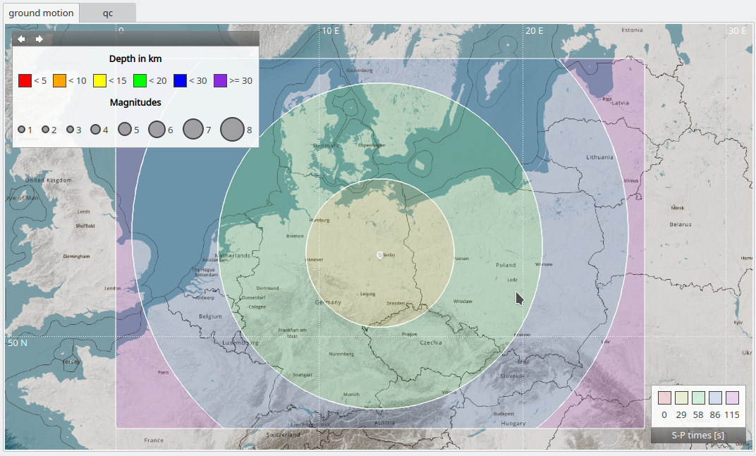
Figure 4: S-P travel-time differences for a POI in Potsdam, Germany and a given travel-time table.
Reports: Station QC and grids
Beyond computing the network performance parameters, npeval can also be used
in order to generate waveform QC report for station which are then archived or
sent to stakeholders by external modules such as GDS [1].
Reports are generated upon
significant changes in QC parameters and/or when triggering of the parameter computation.
An executable script processing the generated reports must defined in
output.script, e.g.
output.script = @DATADIR@/scripts/sendtoGDS.py
The script can be used to archive or disseminate the reports or to process the generated files.
The reports are created in JSON format containing:
Details on the location and the format of the output files generated by the configured methods, if any.
Stream information of stations with information about the station status, available QC parameters and whether it can be considered for grid computation or not. By default only stations with significant updates are reported. To report all stations configure
output.reportAllStations.
Example:
{
  "minimum times": "/tmp/npeval/npeval_times",
  "minimum magnitudes": "/tmp/npeval/npeval_minmag",
  "output format": "GRD",
  "streams": [
    {
      "stream": "CX.PB06..HHZ",
      "significant update": "true",
      "considered": "true",
      "availability": "100",
      "delay": "1.05254",
      "rms": "330.684"
    },
    {
      "stream": "CX.PB09..HHZ",
      "significant update": "true",
      "considered": "false",
      "availability": "100",
      "delay": "1.99461",
      "rms": "1619.25"
    }
  ]
}
The JSON data is provided via stdout to the script in output.script
which is executed. The exit code of the script is evaluated and an error message
is printed if the exit code is not 0.
An example script for processing the JSON data is provided in
@DATADIR@/npeval/tools/npeval-report.sh.example. The raw JSON format
contains no line breaks but it can be converted by other tools, e.g.,
jsonlint for better human readability.
Note
If the station status does not change, the streams item may be empty during the first few grid generations after starting npeval. Initially, grid computations are triggered as more QC parameters arrive for the stations even if the station status does not change.
Considerations
The basic requirement for making an event location and a magnitude estimation is
the detection of seismic phases, e.g., by scautopick [9].
In order to make npeval specific to this phase detector, the involved picker
must be specified by the parameter setupName.
npeval will then only consider stations which have bindings for this module
and for which the data quality control (QC) parameters are within the ranges
defined by the qc.parameters. The station layout is typically read
from the SeisComP database. However, the layout can be overridden by input from
a station file (see section Getting Started).
The minimum number of stations (stations.stationCount)
providing potential arrivals to event location must be met for computing any of
the configured values. An additional quality feature is the maximum allowed
azimuthal gap (stations.maxGap).
Additionally, networks and stations to be considered or to be excluded can be
defined in separate files defined by the parameters stations.file and
stations.exclude-file, respectively.
A typical minimum configuration includes:
Definition of the monitoring region.
Ranges of waveform QC parameters.
The choice of the methods including report generation.
Station setup by
setupNameconsidering pipelines or by a station file (offline application).
A guide for quickly setting up npeval is given in section Getting Started.
Regions
The grid parameters grid.region, grid.spacing and
grid.depths define the considered source locations. Only one region
at a time can be taken into account. Create module aliases for considering
multiple regions. Module aliases can be generated as for
pipelines and configured separately.
Pipe-line systems
In a pipeline system, several instances of a picker, e.g., scautopick [9]
are usually applied independently to different sets of stations. Therefore, npeval
can be configured for separate pipelines by specifying the particular
instance of scautopick (alias) in setupName.
Aliases can be generated and configured separately, e.g., for a region named r1:
seiscomp alias create r1npeval npeval
Quality control parameters
All QC parameters configured by qc.parameters must be available for
the minimum number of stations. The QC parameters
can be received in two ways:
From the database during startup and updating by the parameters received from the messaging system. When reading from the database npeval may by slow during the startup depending on the size of the database.
Only from the messaging system (default). When only using QC parameters from the messaging, the initial grid generation depends on the availability of the QC parameters. It is then typically delayed and the grid may be updated several as QC parameters for more and more stations arrive during the first minutes of operating npeval.
Only stations with QC parameters inside the configured ranges and with a matching
setupName are considered internally for further computations.
Note
Real-time QC parameters are ignored in offline mode.
Triggering and Timing
npeval re-computes the grids by the configured methods or generates reports if the internally considered status of one or more stations changes. This may be when:
npeval is started. The internally considered status is initially set to disabled.
Significant changes in waveform QC parameters are found. That is the QC parameters of stations enter or leave the ranges configured in
qc.parameters.Stations are actively enabled or disabled.
Repeated re-computation in short time intervals may be computational
expensive. Set the parameter grid.update to a reasonable interval to
control the timing and to optimize the load.
Travel-time computation
Depending on the selected method travel times are computed based on the configured travel-time interface, the table and correction parameters.
travelTimes.tableTypeandtravelTimes.table: Type of the interface and name of the travel time tables. Typically, the LOCSAT [3] interface provides faster travel times than libtau. By setting thetravelTimes.tableparameter, customized velocity models can be considered. When choosing LOCSAT, the table file for the P-wave first arrival times must be stored in@DATADIR@/locsat/tables/, for libtau, the velocity profile is stored in@DATADIR@/ttt. Both travel-time interfaces do not consider stations elevations.Correction parameters: Travel-time corrections
 may be applied
based on a configurable average velocity to compensate for station elevation.
The average velocity is typically the P-wave speed at shallow depth as configured in
may be applied
based on a configurable average velocity to compensate for station elevation.
The average velocity is typically the P-wave speed at shallow depth as configured in
travelTimes.velocityCorrection.The velocity
 is applied to the
station elevation
is applied to the
station elevation  and the slowness
  of the first-arrival phase from a grid
point to the station given the travel-time interface and the table configured
by
of the first-arrival phase from a grid
point to the station given the travel-time interface and the table configured
by travelTimes.tableTypeandtravelTimes.table, respectively:
Note
For
 the correction is negative corresponding to a
complex-valued incidence angle. This case may occur if the correction
velocity is larger then the velocity of the upper layer assumed for
computing the travel-time tables or in case of other issues related to the
travel-time interface. Consider checking the travel-time tables/interface
or lower
the correction is negative corresponding to a
complex-valued incidence angle. This case may occur if the correction
velocity is larger then the velocity of the upper layer assumed for
computing the travel-time tables or in case of other issues related to the
travel-time interface. Consider checking the travel-time tables/interface
or lower travelTimes.velocityCorrection. If the computation fails, npeval will consider 0 s for the time correction where the issue occurs.Alternatively, an average station elevation may be compensated for by a correction with respect to sea level. The correction elevation is configured in
travelTimes.elevationCorrection. The travel-time tables must then be computed with respect to this elevation where 0 km depth corresponds to the correction.
Applications
Real-time processing
For running npeval in real time
Make all configurations
Enable and start npeval
seiscomp enable npeval
seiscomp start npeval
or execute on demand
seiscomp exec npeval --debug
Offline processing
npeval can be used in offline processing mode without messaging and real-time data acquisition. Execute npeval on the command line together with other appropriate options
npeval --offline [options]
In this case, waveform QC messages are ignored. This requires the configuration
of times.dataDelay must be configured for computing the
minimum location times and the RMS must be set for
computing the minimum magnitudes. More command-line options
are available.
Designing Networks
In offline processing mode, npeval supports you in designing and optimizing of networks by predicting the performance parameters based on a generic station list:
Configure the required methods
Create a file,
station.txt, containing the station coordinates and QC parameters in the format [NET,STA,LAT,LON,ELEVATION,RMS] where RMS is measured in the unit of counts. Example:CX, PB01, -21.04, -69.49, 320, 150 CX, PB02, -21.32, -69.90, 470, 250
An example script for generating the station table is available in
@DATADIR@/npeval/tools/npeval-make-station-file.sh.example.Run npeval and generate the output
npeval --offline --file stations.txt
Output
File formats
The the output parameters resulting from the considered
methods are stored in the directory and in the file
format configured by output.directory and output.format,
respectively. By default, the output directory is cleared before updating the
files. The supported output formats, defined in output.format are:
BNA files. File suffix: bna.
One sub-directory of
output.directoryis generated per method containing all BNA files. The BNA files contain polylines or closed polygons which can be drawn as layers on map with customized properties [2]. The lines represent minimum values.The layers are drawn at startup of a GUI module, when the
output directoryis either@DATADIR/spatial/vector@or@CONFIGDIR@/spatial/vector. A GUI module must therefore be restarted for considering any file update.CSV comma-separated text file. File suffix: csv.
One file is generated per configured method. Line format:
longitude0,latitude0,value0
longitude1,latitude1,value1
 ...
GRD (default) file (Surfer grid). File suffix: grd.
One file is generated per method. Grid files can be rendered and dynamically updated on maps by the plugin mapmultigrid [6]. GRD is therefore the preferred format. The configuration of the rendering is described in section Grid visualization.
PNG image file. File suffix: png.
One file is generated per method. The colors and contour lines represent minimum values.It is viewable by external image viewers.
Note
By default all files and directories existing in
output.directoryare deleted by npeval when computing any of the desired values. To keep the existing files and directories, uncheckoutput.clean.When running different instances of npeval, configure different output directories which are specific to an instance avoiding to mutually delete the result files.
Grid visualization
Grid files can be dynamically rendered on maps, e.g., of scmv [10] by configuration of the plugin mapmultigrid [6] forming an individual map layer. Multiple grid files can be rendered simultaneously. Upon any changes the grids will be immediately updated on the maps. Read the documentation of mapmultigrid [6] for the complete configuration steps and examples. The debug output of npeval suggests a configuration of color gradients by stops.
Stops and colors
The contours in PNG images and BNA files and the colors (PNG and grids, visualized by the plugin mapmultigrid [6]) represent minimum values. They can be configured by stops which are pairs of computed value and color. The additional attribute “major” or “minor” controls drawing the contour lines in PNG images or the grids.
The stops are configurable in npeval by output.gradient.stops for PNG
or BNA output format. For grid visualization configure the stops parameter
along with the plugin mapmultigrid [6].
A suggestion for the stops configuration stops is printed when running npeval with debug logging output. Example:
npeval --debug

...
  + minimum time: 11.862404 s, maximum time: 163.657563 s from up to 464 stations
  + example configuration of the stops parameter for the plugin mapmultigrid:
  + stops = 10:c02f2f50:"major",52:a5c02f50:"major",94:2fc06750:"major",137:2f6cc050:"major",179:a12fc050:"major"
  + output written to /tmp/npeval/npeval_times.grd
...
Adjust and apply the values to the configuration. The number of suggested stops
can be controlled by the command-line option --suggest-color-intervals.
Example:
npeval --debug --suggest-color-intervals 10
Getting Started
For computing values on grid the recommended minimum configuration is:
Define the events by grid region, depths and spacing:
grid.region,grid.depths,grid.spacing,Configure the stations to consider:
normal processing: Configure
setupNamefor defining the set of stations which has a particular set of bindings. Use global for all stations having global bindings. Setting the value to the instance of scautopick [9] providing the phase picks allows the specific consideration of pipelines.network designing: If no inventory or system setup is available, you may generate a simple text file containing the station names, coordinates and an optional characteristic data RMS value. Format:
network code,station code,latitude,longitude,elevation,RMS
Provide the station file by configuration of :confval:stations.file` or on the command line via
--file.
Define the ranges of waveform QC parameters.
Adjust the minimum number of stations which are expected to provide phase detections:
stations.stationCountconsidering the module creating origins. As an additional quality feature you may set the maximum allowed azimuthal gap bystations.maxGap.Define the output format:
output.format. For BNA or PNG additionally provide the stops:output.gradient.stopsConfigure the methods to be considered:
times.*andminimumMagnitude.*.For specific points of interest configuring the POIs parameters,
POIs.
For sending reports on significant changes of station parameters and updates configure:
The waveform QC parameters to be considered:
qc.parameters.The report script to handle the reports:
output.script.
Examples
Real-time processing on the command line considering waveform QC messages:
npeval --region 80,150,-20,30 --delta 1 -d localhost/seiscomp
Real-time processing on the command line considering constant RMS (nm/s):
npeval -d localhost/seiscomp --rms 500
Offline processing on the command line with a station file and a station exclude file:
npeval --offline --file stations.ini --region 21,27,62,67 --exclude-file stat-excl.ini --debug
Offline processing on the command line with a station file and station RMS in nm/s overwriting all other RMS values:
npeval --offline --file stations.ini --rms 300
Module Configuration
etc/defaults/global.cfgetc/defaults/npeval.cfgetc/global.cfgetc/npeval.cfg~/.seiscomp/global.cfg~/.seiscomp/npeval.cfgnpeval inherits global options.
Note
Modules/plugins may require a license file. The default path to license
files is @DATADIR@/licenses/ which can be overridden by global
configuration of the parameter gempa.licensePath. Example:
gempa.licensePath = @CONFIGDIR@/licenses
- setupName
Default:
scautopickType: string
List of configuration setup names used for the initial setup of the active station list. Use commas to separate names. E.g. in pipelines use the names of all modules contributing picks.
"scautopick": consider all stations with scautopick bindings and the streams defined therein.
"default" or "global": consider all stations with global bindings and the streams defined therein.
Note
qc.* Waveform quality control (QC) parameters. Configure npeval to subscribe to the basic message groups, e.g. QC, CONFIG.
- qc.parameters
Type: list:string
Range:
-Inf:InfDefine QC parameters to observe. Each parameter is associated with a value range. If any of the defined ranges is exceeded the corresponding station is disabled. For the ranges use ‘-Inf,Inf’ if no upper or lower limits shall exist.
Typical parameters: rms, latency, delay, availability, gaps count, overlaps count, timing quality, offset, spikes count. Read $SEISCOMP_ROOT/etc/defaults/npeval.cfg for examples.
scqc must be running in parallel.
- qc.useDatabase
Default:
falseType: boolean
Load QC parameters from the database during startup. Setting to true may slow down the start up.
Note
stations.* Parameters controlling the stations to be considered.
- stations.stationCount
Default:
4Type: uint
Minimum number of stations that have an arrival for starting the calculations. This mimics the confiugration of the phase associator, e.g., scanloc or scautoloc.
- stations.maxGap
Default:
360.0Unit: deg
Type: double
Range:
-1:InfMaximum allowed azimuthal gap between adjacent stations for starting calculations. If the gap is larger than configured, more stations than configured by "stations.stationCount" are requested.
The gap is only tested when "stations.maxGap " < 360.0.
The parameter only applies to the minimum time method.
- stations.file
Type: file
Name of CSV file to read station information from instead of considering "setupName". Use the option for designing new networks without inventory and global bindings. One line per station.
Format: NET,STA,LAT,LON,ELEVATION,RMS
RMS (nm/s) is optional and required for minimum magnitude calcuation in offline mode.
- stations.excludeFile
Type: file
Name of a station blocklist file. Each line has the format [NET].[STA] supporting wildcards. Example:
CX.PB01
GE.*
Note
grid.* Parameters controlling the source region grid and the update interval. Grid points represent hypocenters.
- grid.region
Default:
80.0,150.0,-20.0,30.0Unit: deg
Type: list:float
Horizontal bounding box for selecting the considered region: LonMin,LonMax,LatMin,LatMax. Required parameter.
- grid.spacing
Default:
1.0Unit: deg
Type: double
Horizontal grid spacing for assuming events.
- grid.depths
Default:
10.0Unit: km
Type: list:double
Source depths. Use comma separation for a list of values.
- grid.update
Default:
60Unit: s
Type: double
Range:
1:InfMinimum time interval between 2 updates. Values < 1 are set to 1.
Note
output.* Output control parameters.
- output.directory
Default:
/tmp/npevalType: directory
Directory for writing result files. The directory will be created if not existing. The file format is configured in "output.format"
Recommendation for BNA files: @DATADIR@/spatial/vector/npeval.
- output.clean
Default:
trueType: boolean
Clean output directory before writing new result files.
- output.format
Default:
GRDType: string
Values:
BNA,CSV,GRD,PNGFormat of result files written to "output.directory".
- output.size
Default:
1280x1024Unit: px
Type: string
PNG image size.
- output.script
Type: file
Path to the executable script file which is executed when the network parameters are computed. Station reports and output result files are provided to the script.
- output.reportAllStations
Default:
falseType: boolean
Report all stations and not just those with significant updates. "output.script" must be configured for this parameters to be effective.
- output.gradient.discrete
Default:
trueType: boolean
Setting this parameter to true enables color interpolation.
- output.gradient.stops
Default:
30.00:ff00fa,60.00:f25ffb,90.00:e483fc,120.00:d79cfd,150.00:c9aefe,180.00:9fd7ff,210.00:93dfff,240.00:84e8ff,270.00:6df2ff,300.00:49fdff,600.00:20dbdb,900.00:11b4b7,1200.00:03939aType: gradient
The colors at given levels for drawing PNG images. Use hexadecimal color values.
Note
travelTimes.* Parameters for calculating the travel times which are used by the methods minimum time, minimum magnitude and S-P travel times.
- travelTimes.tableType
Default:
LOCSATType: string
Values:
libtau,LOCSAT,homogeneousType of travel-time table (interface).
- travelTimes.table
Default:
iasp91Type: string
Name of travel-time table (interface profile).
- travelTimes.velocityCorrection
Default:
-1.0Unit: km/s
Type: double
Correction velocity added to travel times in order to account for station elevation which is currently not accounted for by LOCSAT and libtau. Applying a positive value deactivates "elevationCorrection"
- travelTimes.elevationCorrection
Default:
0.0Unit: km
Type: double
An elevation of stations added to the event depth for computing travel times. The travel-time table should start at this elevation correction. Currently, LOCSAT and libtau do not correct for sensor elevation.
The parameter is deactivated by "velocityCorrection".
Note
times.* Parameters for calculating the minimum times to locate events by a network.
- times.compute
Default:
trueType: boolean
Allow computing the minimum times.
- times.file
Default:
npeval_timesType: string
Basename of output file(s) for the times grid.
- times.dataDelay
Default:
-1.0Unit: s
Type: float
Data delay to be added to computed travel times.
-1.0 - get automatically from QC messages per station.
- times.processingDelay
Default:
5.0Unit: s
Type: float
Data processing time to be added to computed travel times. The amount must considers time windows for AIC used by scautopick and mB when using scautoloc with mB amplitudes. The value must be therefore be changed when adjusting those window lengths.
Note
minimumMagnitude.* Parameters for calculating the minimum magnitude of events that can be detected by a network.
- minimumMagnitude.compute
Default:
falseType: boolean
Allow computing the expected minimum magnitude.
- minimumMagnitude.file
Default:
npeval_minmagType: string
Basename of output file(s) for the magnitudes grid.
- minimumMagnitude.type
Default:
LFType: string
Values:
LF,MDD,GMPEType of amplitude calculation:
LF: low-frequency approximation
MDD: magnitude-detection distance
GMPE: GMPE (trial only).
- minimumMagnitude.magMin
Default:
2.0Type: float
Minimum earthquake magnitude to be tested. Step size to maximum: 0.1.
- minimumMagnitude.magMax
Default:
5.0Type: float
Maximum earthquake magnitude to be tested.
- minimumMagnitude.magStep
Default:
0.2Type: float
Magnitude step.
- minimumMagnitude.minSnr
Default:
5Type: float
Minimum signal-to-noise ratio at the station to accept a magnitude.
Note
minimumMagnitude.lowFrequency.* Values for calculating the low-frequency amplitude. The method is used when “minimumMagnitude.type” = LF. Default values are from the ak135 standard Earth model at 10 km depth. The method requires travel times considering the parameters configured in the section “travelTime”.
- minimumMagnitude.lowFrequency.vp
Default:
5.8Unit: km/s
Type: float
Range:
0:InfP-wave velocity at the hypocentre.
- minimumMagnitude.lowFrequency.vs
Default:
3.2Unit: km/s
Type: float
Range:
0:InfS-wave velocity at the hypocentre. vs = vp/sqrt(3) if not set.
- minimumMagnitude.lowFrequency.rho
Default:
2.6Unit: g/cm^3
Type: float
Density at the hypocentre.
- minimumMagnitude.lowFrequency.sigma
Default:
10Unit: bar
Type: float
Stress drop due to the earthquake.
- minimumMagnitude.lowFrequency.qp
Default:
500Type: float
Qp, seismic attenuation along the ray given by the quality factor for P waves.
Note
minimumMagnitude.magnitudeDetectionDistance.* Values for calculating the expected magnitude based on based on the regression of M = b*log10(distance) + a * distance + c. Defaults are from Valtonen et al. (2013).
- minimumMagnitude.magnitudeDetectionDistance.a
Default:
0.001514Unit: 1/km
Type: float
The a parameter in the regression equation.
- minimumMagnitude.magnitudeDetectionDistance.b
Default:
0.9327Type: float
The b parameter in the regression equation.
- minimumMagnitude.magnitudeDetectionDistance.c
Default:
-1.306Type: float
The c parameter in the regression equation.
Note
nStations.* Parameters for calculating the number of stations available for detecting events on a grid.
- nStations.compute
Default:
falseType: boolean
Allow computing the number of stations.
- nStations.maximumDistance
Default:
0Unit: km
Type: float
The maximum hypocentral distance to consider a station. This parameter will be ignored if ‘nStations.magnitude’ > -10.
- nStations.magnitude
Default:
-10Type: float
The magnitude from which to compute the maximum distance. Values <= -10 will disable this parameter and for the distance is ‘nStations.maximumDistance’ is assumed. For estimating a distance, the parameters of the MDD method are assumed.
Note
POIs.* Compute paramters for individual points of interest (POI).
- POIs.file
Default:
npeval_poiType: string
Base name of output file(s) for the POIs grid. The profile name will be appended.
- POIs.poiProfiles
Type: list:string
Registration of POI profiles. An empty list disables all POIs.
Note
POIs.profiles.$name.*
$name is a placeholder for the name to be used and needs to be added to poiProfiles to become active.
poiProfiles = a,b
POIs.profiles.a.value1 = ...
POIs.profiles.b.value1 = ...
# c is not active because it has not been added
# to the list of poiProfiles
POIs.profiles.c.value1 = ...
- POIs.profiles.$name.latitude
Unit: deg
Type: double
Latitude.
- POIs.profiles.$name.longitude
Unit: deg
Type: double
Longitude.
- POIs.profiles.$name.elevation
Unit: km
Type: double
Elevation above above sea level (WGS84).
- POIs.profiles.$name.computeSP
Default:
falseType: boolean
Select to compute S-P travel time differences.
Command-Line Options
Generic
- -h, --help
Show help message.
- -V, --version
Show version information.
- --config-file file
The alternative module configuration file. When this option is used, the module configuration is only read from the given file and no other configuration stage is considered. Therefore, all configuration including the definition of plugins must be contained in that file or given along with other command-line options such as --plugins.
- --plugins arg
Load given plugins.
- -D, --daemon
Run as daemon. This means the application will fork itself and doesn’t need to be started with &.
Verbosity
- --verbosity arg
Verbosity level [0..4]. 0:quiet, 1:error, 2:warning, 3:info, 4:debug.
- -v, --v
Increase verbosity level (may be repeated, e.g., -vv).
- -q, --quiet
Quiet mode: no logging output.
- --print-component arg
For each log entry print the component right after the log level. By default the component output is enabled for file output but disabled for console output.
- --component arg
Limit the logging to a certain component. This option can be given more than once.
- -s, --syslog
Use syslog logging backend. The output usually goes to /var/lib/messages.
- -l, --lockfile arg
Path to lock file.
- --console arg
Send log output to stdout.
- --debug
Execute in debug mode. Equivalent to --verbosity=4 --console=1 .
- --trace
Execute in trace mode. Equivalent to --verbosity=4 --console=1 --print-component=1 --print-context=1 .
- --log-file arg
Use alternative log file.
Stations
- --file arg
Overrides configuration parameter
stations.file.
- --exclude-file arg
Overrides configuration parameter
stations.exclude-file.
- --skip arg
Default:
0.0Unit: %
Type: double
Randomly skip the given percentage of stations.
Output
- -f, --format arg
Overrides configuration parameter
output.format.
- --directory arg
Overrides configuration parameter
output.directory.
- --size arg
Overrides configuration parameter
output.size.
- --no-clean
Do not clean output directory before writing new output. Otherwise the output directory will be cleaned.
- --clean
Overrides configuration parameter
output.clean.Overrides --no-clean.
- --suggest-color-intervals arg
Default:
5Type: int
The number of contour intervals and related color to suggest together along with debug logging output.
Region
- --region arg
Overrides configuration parameter
grid.region.
- --spacing arg
Overrides configuration parameter
grid.spacing.
- --depths arg
Overrides configuration parameter
grid.depths.For series use --depths 10 --depths 20 …
Times
- --dataDelay arg
Overrides configuration parameter
times.dataDelay.
- --procDelay arg
Overrides configuration parameter
times.processingDelay.
- -c, --station-count arg
Overrides configuration parameter
stations.stationCount.
- --times-file arg
Overrides configuration parameter
times.file.