
Filter Grammar
SeisComP supports string-based filter definitions. This section covers available filters and their parameters.
The filter definitions support SeisComP filters and building filter chains (operator >> or ->) as well as combining them with basic mathematical operators. Filter or the first filter in a filter chain is always applied to the raw, uncorrected data. Use brackets () to apply the operations within before the one outside.
Mathematical operators are:
+ : addition
- : subtraction
* : multiplication
/ : division
^ : power / exponentiation
|. | : absolute value.
A special mathematical operator is a negative value replacing a positive frequency value, e.g., in Butterworth filters (see Section List of filters). The modulus of the frequency value is multiplied by the sample rate of the waveforms to which it is applied. The resulting value defines the frequency the filter is configured with. Note, -0.5 defines the Nyquist frequency of the data. Negative values can be applied for defining frequencies dynamically based on sample rate.
Example:
Data with a sample rate of 100 Hz shall be low-pass filtered at 80% of the
Nyquist frequency by a Butterworth low-pass filter, BW_LP. A
value of -0.4 corresponds to 80% of the Nyquist frequency. The filter can be
specified as BW_LP(3,-0.4).
Note
Filters in SeisComP are recursive allowing real-time application. Therefore, filter artefacts, e.g. ringing, are always visible at the beginning of the traces or after data gaps.
Example
A(1,2)>>(B(3,4)*2+C(5,6,7))>>D(8)
where A, B, C and D are different filters configured with different parameters. In this example a sample s is filtered to get the final sample sf passing the following stages:
filter sample s with A: sa = A(1,2)(s)
filter sa with B: sb = B(3,4)(sa)
sb = sb * 2
filter sa with C: sc = C(5,6,7)(sa)
add sb and sc: sbc = sb + sc
filter sbc with D: sf = D(8)(sbc)
sf = final sample.
The default filter applied by scautopick for making detections is
RMHP(10) >> ITAPER(30) >> BW(4,0.7,2) >> STALTA(2,80)
It first removes the offset. Then an ITAPER of 30 seconds is applied before the data is filtered with a fourth order Butterworth bandpass with corner frequencies of 0.7 Hz and 2 Hz. Finally an STA/LTA filter with a short-time time window of 2 seconds and a long-term time window of 80 seconds is applied.
To apply mathematical operations on original waveforms use self(), e.g.:
self()^2>>A(1,2)
Test filter strings
Filters can be conveniently tested without much configuration. To perform such tests
Open a simple graphical text editor, e.g. gedit, pluma or kwrite and write down the filter string.
Mark / highlight the filter string and use the mouse to drag the filter string onto the waveforms.
Observe the differences between filtered and unfiltered waveforms.
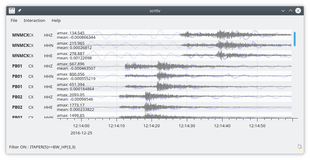
scrttv with raw (blue) and filtered (black) data. The applied filter string is shown in the lower left corner.
List of filters
Multiple filter functions are available. Filters may take parameters as
arguments. If a filter function has no parameter, it can be given either with
parentheses, e.g. DIFF(), or without, e.g.
DIFF.
Warning
All frequencies passed by parameters to filters must be below the Nyquist frequency of the original signal. Otherwise, filtering may result in undesired behavior of modules, e.g., stopping or showing of empty traces.
- AVG(timespan)
Calculates the average of preceding samples.
- Parameters:
timespan – Time span to form the average in seconds
- BPENV(center-freq, bandwidth, order)
Butterworth bandpass filter combined with envelope computation.
This is a recursive approximation of the envelope. It depends on the bandpass center frequency being also the dominant frequency of the signal. Hence it only makes sense for bandpass filtered signals. Even though bandwidth and order may be changed it is recommended to use the defaults.
- Parameters:
center-freq – The center frequency of the passband in Hz. Negative values define the frequency as -value * sample rate.
bandwidth – The filter bandwidth in octaves (default is 1 octave)
order – The filter order of the bandpass (default is 4)
- BW(order, lo-freq, hi-freq)
Alias for the
Butterworth band-pass filter, BW_BP.
- BW_BP(order, lo-freq, hi-freq)
Butterworth bandpass filter (BW) realized as a causal recursive IIR (infinite impulse response) filter. An arbitrary bandpass filter can be created for given order and corner frequencies.
- Parameters:
order – The filter order
lo-freq – The lower corner frequency as 1/seconds. Negative values define the frequency as -value * sample rate.
hi-freq – The upper corner frequency as 1/seconds. Negative values define the frequency as -value * sample rate.
- BW_BS(order, lo-freq, hi-freq)
Butterworth band stop filter realized as a causal recursive IIR (infinite impulse response) filter suppressing amplitudes at frequencies between lo-freq and hi-freq.
- Parameters:
order – The filter order
lo-freq – The lower corner frequency as 1/seconds. Negative values define the frequency as -value * sample rate.
hi-freq – The upper corner frequency as 1/seconds. Negative values define the frequency as -value * sample rate.
- BW_HP(order, lo-freq)
Butterworth high-pass filter realized as a causal recursive IIR (infinite impulse response) filter.
- Parameters:
order – The filter order
lo-freq – The corner frequency as 1/seconds. Negative values define the frequency as -value * sample rate.
- BW_HLP(order, lo-freq, hi-freq)
Butterworth high-low-pass filter realized as a combination of
BW_HP()andBW_LP().- Parameters:
order – The filter order
lo-freq – The lower corner frequency as 1/seconds. Negative values define the frequency as -value * sample rate.
hi-freq – The upper corner frequency as 1/seconds. Negative values define the frequency as -value * sample rate.
- BW_LP(order, hi-freq)
Butterworth low-pass filter realized as a causal recursive IIR (infinite impulse response) filter.
- Parameters:
order – The filter order
hi-freq – The corner frequency as 1/seconds. Negative values define the frequency as -value * sample rate.
- CUTOFF(delta)
Sets the value of the current sample to the mean of the current and the previous sample when the difference between the two exceeds delta. Otherwise, the original value is retained.
- Parameters:
delta – The threshold for forming the average.
- DIFF()
Differentiation filter realized as a recursive IIR (infinite impulse response) differentiation filter.
The differentiation loop calculates for each input sample s the output sample s':
s' = (s-v1) / dt
v1 = s;
- DT()
Replaces each input sample with the sampling interval of the current sample. This is a shortcut for
1/SRbut more efficient as the division has to be done only once and not once per input sample. The output unit is seconds.
- DURATION(trigger_on, trigger_off)
Replaces the input samples with the trigger duration. The duration is computed as the time between trigger_on and trigger_off. Outside the trigger, the filter outputs zero.
- INT([a = 0])
Integration filter realized as a recursive IIR (infinite impulse response) integration filter. The weights are calculated according to parameter a in the following way:
a0 = ((3-a)/6) * dt
a1 = (2*(3+a)/6) * dt
a2 = ((3-a)/6) * dt

b0 = 1
b1 = 0
b2 = -1
The integration loop calculates for each input sample s the integrated output sample s':
v0 = b0*s - b1*v1 - b2*v2
s' = a0*v0 + a1*v1 + a2*v2
v2 = v1
v1 = v0
- Parameters:
a – Coefficient a.
- ITAPER(timespan[, offset = 0])
A one-sided cosine taper applied when initializing the filter, e.g. at the beginning of the data or after longer gaps.
- Parameters:
timespan – The length of the taper in seconds
offset – The offset in counts removed from the data records before applying the taper. Optional parameter.
- MAX(timespan)
Computes the maximum within the timespan preceding the sample.
- Parameters:
timespan – The timespan to measure the maximum in seconds
- MEDIAN(timespan)
Computes the median within the timespan preceding the sample. Useful, e.g. for despiking. The delay due to the filter may be up to its timespan.
- Parameters:
timespan – The timespan to compute the median in seconds
- MIN(timespan)
Computes the minimum within the timespan preceding the sample.
- Parameters:
timespan – The timespan to measure the minimum in seconds
- RM(timespan)
A running mean filter computing the mean value within timespan. For a given time window in seconds the running mean is computed from the single amplitude values and set as output. This computation is equal to
RHMPwith the exception that the mean is not subtracted from single amplitudes but replaces them.RMHP = self-RM
- Parameters:
timespan – The timespan to measure the mean in seconds
- RMHP(timespan)
A high-pass filter realized as running mean high-pass filter. For a given time window in seconds the running mean is subtracted from the single amplitude values. This is equivalent to high-pass filtering the data.
Running mean high-pass of e.g. 10 seconds calculates the difference to the running mean of 10 seconds.
- Parameters:
timespan – The timespan to measure the mean in seconds
- RND(mean, stddev)
A random signal generator with Gaussian normal distribution. It replaces input samples with the new signal. Use RND() with the operator ‘+’ for adding the random signal to some data. Example: (BW(3,0.7,2) + RND(0,10))>>STALTA(2,80)
- Parameters:
mean – The mean value of the normal distribution
stddev – The standard deviation of the normal distribution
- RUD(minimum, maximum)
A random signal generator with uniform distribution. It replaces input samples with the new signal. Use RUD() with the operator ‘+’ for adding the random signal to some data. Example: (BW(3,0.7,2) + RUD(-10,10))>>STALTA(2,80)
- Parameters:
minimum – The minimum value of the uniform distribution
maximum – The maximum value of the uniform distribution
- self()
The original data itself.
- SM5([type = 1])
A simulation of a 5-second seismometer.
- Parameters:
type – The data type: either 0 (displacement), 1 (velocity) or 2 (acceleration)
- SR()
Replaces each input sample with the sampling rate of the current sample. The output unit is 1/seconds.
- STALTA(sta, lta)
A STA/LTA filter is the ratio of a short-time amplitude average (STA) to a long-time amplitude average (LTA) calculated continuously in two consecutive time windows. This method is the basis for many trigger algorithm. The short-time window is for detection of transient signal onsets whereas the long-time window provides information about the actual seismic noise at the station.
- Parameters:
sta – Length of short-term time window in seconds
lta – Length of long-term time window in seconds. The time window ends with the same sample as sta.
- STALTA2(sta, lta, on, off)
The
STALTA()implementation where LTA time window is kept fixed between the time the STA/LTA ratio exceeds on and falls below off.- Parameters:
sta – Length of short-term time window in seconds
lta – Long-term time window ending with the same sample as sta
on – STA/LTA ratio defining the start of the time window for fixing LTA.
off – STA/LTA ratio defining the end of the time window for fixing LTA.
- SUM(timespan)
- Parameters:
timespan – The timespan to be summed up in seconds
Computes the amplitude sum of the timespan preceding the sample.
- WA([type = 1[, gain = 2080[, T0 = 0.8[, h = 0.7]]]])
The simulation filter of a Wood-Anderson seismometer. The data format of the waveforms has to be given for applying the simulation filter (displacement = 0, velocity = 1, acceleration = 2), e.g., WA(1) is the simulation on velocity data.
- Parameters:
type – The data type: 0 (displacement), 1 (velocity) or 2 (acceleration)
gain – The gain of the Wood-Anderson response
T0 – The eigen period in seconds
h – The damping constant
- WWSSN_LP([type = 1])
The instrument simulation filter of a World-Wide Standard Seismograph Network (WWSSN) long-period seismometer.
- Parameters:
type – The data type: 0 (displacement), 1 (velocity) or 2 (acceleration)
- WWSSN_SP([type = 1])
Analog to the
WWSSN_LP(), the simulation filter of the short-period seismometer of the WWSSN.- Parameters:
type – The data type: 0 (displacement), 1 (velocity) or 2 (acceleration)

