Polarity Picker
This plugin provides the polarity pickers POLAIC and POLARITY which are capable of determining the first motion direction of the onset automatically.
Overview
The plugin picker-plugins provides two ways to determine the first motion of a P pick automatically. First, the POLAIC utilizes the picker interface and second, the POLARITY the feature-extraction interface FX. Both work almost identical as they use the same internal algorithms to determine the pick polarity. The only difference is the interface and therefore when the polarity picker is started.
In general, the polarity is either set to positive or negative if the
polarity was determined successfully, or to undecidable if the intern
algorithms cannot determine it uniquely.
The polarity is left unset if any intern algorithms fail or if configuration
criteria, like minSNR, are not fulfilled.
POLAIC
The POLAIC is built on top of the default AIC algorithm used to refine the P pick. In addition to the standard AIC behavior, the POLAIC tries to identify the first motion direction by applying one or multiple algorithms.
Note
The AIC settings are automatically read from the picker.AIC.*
and cannot be redefined in the POLAIC configuration section.
Picks made by using POLAIC can be identified:
In the method column of the arrival table in the Location tab of scolv [1],
In the picker window from the letter within brackets following a phase type (<P>),
In the picker window from the method hint which appears when hovering over a pick.
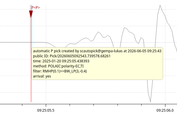
Read the pick method (scolv picker window) to check the applied method which was used to create a pick polarity.
POLARITY
The POLARITY uses the FX interface to determine the pick polarity after a pick is made.
Picks made by POLARITY can only be identified in the picker window from the comment which appears when hovering over a pick.
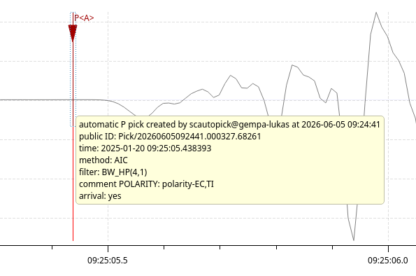
Read the pick comment (scolv picker window) to check the applied method which was used to create a pick polarity.
Picker configuration
Plugin loading: Add the plugin polpicker to the configuration of scautopick or the global module configuration for making use of POLAIC or POLARITY:
plugins = ${plugins}, polpicker
Module parameters: Activate the POLAIC by changing the name of the
pickerin the module configuration of scautopick:picker = "POLAIC"
or to use the POLARITY set the
fxvalue in the scautopick configuration:fx = "POLARITY"
Bindings parameters: Configure the POLAIC parameters under
pickerin global section of the bindings of scautopick. An example:picker.POLAIC.minSNR = 20 picker.POLAIC.algorithms = EC-env,TI picker.POLAIC.decider = polarity picker.POLAIC.noiseBegin = -1.0 picker.POLAIC.signalBegin = -0.67 picker.POLAIC.signalEnd = 0.5 picker.POLAIC.filter = "RMHP(0.1)" picker.POLAIC.useTime = true picker.POLAIC.enableLinearDetrend = false picker.POLAIC.disableAIC = false
or for POLARITY under
fx:fx.POLARITY.minSNR = 20 fx.POLARITY.algorithms = EC-env,TI fx.POLARITY.decider = polarity fx.POLARITY.noiseBegin = -1.0 fx.POLARITY.signalBegin = -0.67 fx.POLARITY.signalEnd = 0.5 fx.POLARITY.filter = "RMHP(0.1)" fx.POLARITY.useTime = true fx.POLARITY.enableLinearDetrend = false
Repicker in scolv: In addition, the POLAIC is available as a repicker in the scolv picker window. In the repicker drop-down menu of the scolv picker, the entry POLAIC should appear. Enable ‘P picking’ and press ‘R’ to automatically repick with POLAIC. Make sure the plugin in loaded either in the global module or scolv configuration:
plugins = ${plugins}, polpicker
Hints for parameter configuration ordered by its suggested priority to tune:
Priority |
Parameter |
Hints |
|---|---|---|
High |
Depending on the noise level the SNR needs to be adjusted. For robust and confident polarities use |
|
High |
|
The time parameter need to be adjusted based on sampling rate, (usual) period of the phase onset and the uncertainty of the initial picktime. Lower sampling rates need longer time windows to have enough samples to initialize internal methods. In general, the noise window (between The default values were calibrated on 100 Hz data. Initial testing suggested a reasonable |
Medium |
See Algorithms for a detailed explanation of the available algorithms. In general, defining multiple algorithms should increase the confidence of the correctness of the polarity with the drawback of missing out on some polarities. Recommended combinations:
|
|
Medium |
Is only used if multiple |
|
Low |
Although polarities should be picked on unfiltered waveforms, the algorithms might benefit from applying filters that remove noise or precursor artifacts. Depending on the presumed dominant frequency of the signal, low-frequent noise (e.g. microseism) might be filtered out by using a high-pass filter. For example, the filter RMHP(0.1) might not significantly distort the phase of the incoming P phase. For picking polarities on phases that have similar frequencies compared to the sensor sample-rate, precursor artifacts might be visible. To remove their influence, a low-pass filter, e.g. BW_LP(3,-0.4), might be useful. |
|
Low |
Only valid for algorithm DP-fixed: Fixed period of the expected dominant waves for the first motion. |
|
Low |
Most algorithms, except DP and DP-fixed, are capable of determining an own phase onset time belonging to the predicted polarity. Usually, if the polarity is correct, the pick time truly improves. But there are special cases, highly depending on the waveform data before the actual pick, in which the pick time quality might decrease. |
|
Low |
|
On linearly detrended traces the results of the algorithms might stabilize. |
Low |
Disabling the AIC picker might be useful if |
Algorithms
Determining the first motion correctly can become a challenging task and may result in non-unique solutions. Therefore the plugin provides a set of algorithms that try to determine the first motion based on different approaches.
The simplest approach is measuring the gradient between the pick and its next sample. As the POLAIC and POLARITY are embedded in an automatic processing chain and each automatic pick usually has an uncertainty that is higher than a few samples, the reference pick might not be accurate enough to reliably apply the simple gradient method. Further, the waveform may be affected by high noise levels (either low- or high-frequent), which may make the absolute measurement of the gradient incorrect for such cases.
Instead, more robust algorithms were implemented. Those assume an uncertainty of the initial triggering pick and, thus, consider a larger time window around the pick. Still each algorithm has its drawbacks and might only be useful for certain types of waveform data.
Besides determining the first motion, most of the available algorithms
are capable of refining the pick time by determining the sample that
most-likely corresponds to the polarity onset.
Configure the parameter useTime to enable/disable the pick time
refinement.
TI (threshold increaser)
The idea of this algorithm is that the polarity is the first stable amplitude that exceeds the noise. The polarity amplitude is determined by the amplitude that crosses two consecutively increased thresholds.
As the thresholds are drawn horizontally (based on the noise level), it is important that the waveform data does not include any trends and the (long-term, low-frequent) noise level should be significantly smaller than the signal level (see figures below).
Advantages:
Simplicity of the algorithm
Reliable for strong, impulsive first motions
Potential disadvantages:
Does not work with large low-frequent noise and trends in the data
Might miss weak first motions
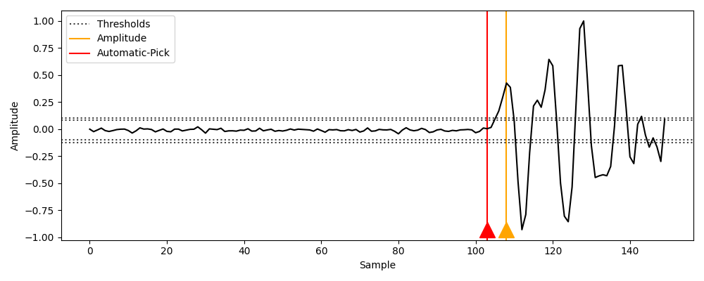
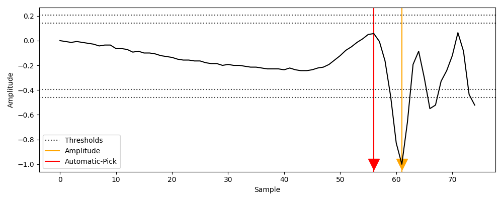
Two examples showing the basic idea of the algorithm. Dashed, horizontal
lines represent the increasing thresholds.
The yellow pick represents the amplitude that is responsible for the polarity
decision, while the red pick is the position of the final pick if
useTime is true.
For data where the signal is large compared to the background noise (top),
the algorithm performs well. For example, if the waveform is highly
influenced by low-frequent noise (bottom), the threshold approach is not
suitable anymore and might produce erroneous polarities.
EC (extrema comparer)
The idea of this algorithm is that the polarity defining extremum is significantly larger than the previous extremum. The contrast between each pair of consecutive extrema is calculated. The extremum with the largest contrast to its previous extremum defines the polarity. To stabilize the results, the algorithm considers only extrema within a most-likely time window around the P onset and calculates for each extrema pair a local mean level before determining the amplitude contrast. The latter results in a more robust determination of the polarity, especially in low-frequent noise environments (see figures below).
Advantages:
More robust in noisy environments
Reliable for strong amplitude first motions
Has derivatives tackling certain use cases
Potential disadvantages:
Might not work on too smooth data
Might miss weak first motions
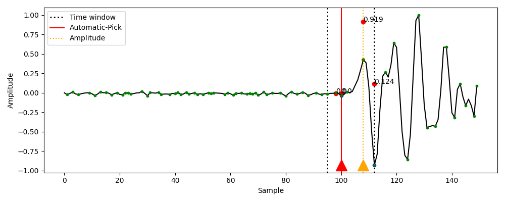
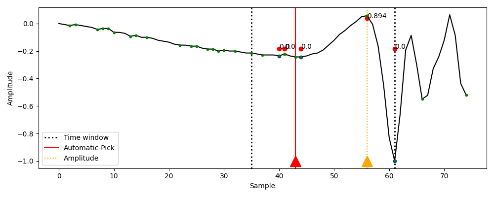
Two examples showing the basic idea of the algorithm. Green dots mark all
extrema, whereas red dots mark only the relevant extrema, which lie in the
predicted most-likely arrival time window (vertical, dotted lines).
Next to each red dot is the confidence value, the extremum with the highest
value determines the polarity.
The yellow pick represents the amplitude that is responsible for the polarity
decision, whereas the red pick is the position of the final pick if
useTime is true.
The approach is capable of finding the correct polarities for data with
large SNR (top) as well as for data significantly influenced by
low-frequent noise (bottom).
To tackle some of its limitations, the algorithm has some extensions.
For example, add the env extension by replacing
EC with EC-env.
Available extensions:
EC-env: combines amplitude ratios for an envelope trace with the original trace ratios - enhances the detection quality of first motions with small amplitudesEC-DP: applies a weighting based on a period depending time difference to the pick - prefers polarities close to the initial pickEC-noend: there is no end time window restriction by the internal algorithm - helps if the initial pick is too early
and combinations: EC-env-noend,
EC-DP-env and
EC-DP-noend
DP (dominant period)
In the first step, the dominant period is determined or, for the fixed mode,
read from the configuration (picker.POLAIC.period or
fx.POLARITY.period).
Based on the period value, a time window around the pick is calculated.
The final polarity is defined by the average slope of the time window.
Configure DP-fixed for the fixed method.
Decider
It is possible to use multiple algorithms simultaneously on the same pick by
providing multiple entries in picker.POLAIC.algorithms or
fx.POLARITY.algorithms.
Each algorithm determines polarity and sample individually.
The final polarity that will be associated to the pick needs to be determined
based on the outcome of all algorithms.
For that reason several decider algorithms are available:
polarity: sets the polarity only if all algorithms predict the same polarity, otherwise sets it to undecidablesample: sets the polarity only if all algorithms predict the same sample as phase onset (as most algorithms are capable of refining the pick time), otherwise sets it to undecidablemajority: sets the polarity to the value of the majority of the results, the polarity is set to undecidable if it is a draw
Note
If only one single algorithm is used, the decider is skipped and the polarity is directly determined by the algorithm.
Validation on test sets
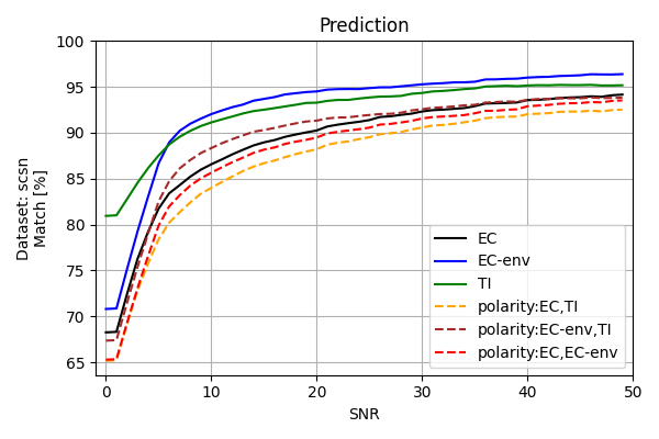
The performance of the algorithms have been validated by using publicly available first motion datasets. From the Instance data set (Michelini et al. [8]) 19995 and from the SCSN data set (Ross et al. [10]) 13310 manually picked polarities were used. The figures below show the performance of three algorithms (by POLAIC/POLARITY) and their combinations against the polarities of the validation data sets.
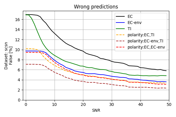
The overall prediction capability is visible in the figures a) and c). The automatic picker achieve a high matching score with more than 90% correctly predicted polarities. As expected, with increasing SNR the prediction capability increases. Single algorithms usually perform better than combinations, as combinations may set the polarity to undecidable, if discordant, which will counts as a wrong prediction. The figures b) and d) show the percentage of relevant false predictions, by only considering picks for which the automatic prediction did not predict undecidable. This should show how robust an algorithm (or combination) is against predicting the wrong impactful polarity (either up or down). Here the combinations tend to perform better, as they predict more often undecidable, if discordant. An undecidable polarity should not have any significant or erroneous impact.
To summarize, combinations of algorithms may result in fewer polarities (up or down) but the probability of the correctness is higher in comparison to using only single algorithms.
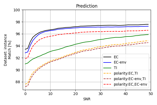
a: The plots show the matching percentage between predictions by selected algorithms and the Instance data set [8] for all data points with at least at certain SNR value.
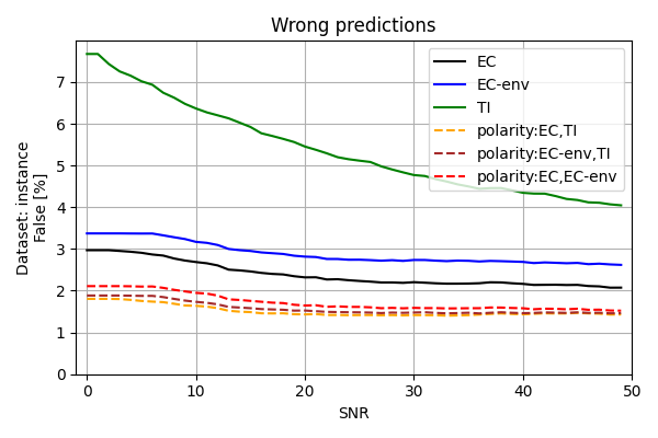
b: The plots show the mismatch percentage between predictions by selected algorithms and the Instance data set [8] for data points with at least at certain SNR value and for points the prediction algorithms did not chose undecidable.